


Next: Step 2: Calculation of
Up: Example 1: Stabilization of
Previous: Example 1: Stabilization of
Contents
For  , a Hall basis for
 is first constructed by invoking
  :=phb(3,4), which yields as a list of 32 elements, conveniently denoted by
  ,
,
 , where the set of multi-
 contains all Hall words of length not exceeding four using the alphabet
  ; see Remark 3.1.
To evaluate the images
; see Remark 3.1.
To evaluate the images
 ,
, of the elements in the Hall basis the vector fields
,
, of the elements in the Hall basis the vector fields  are declared as symbolic expressions in Maple, and the function calcLB is invoked, remembering that
 ,
,  .
The 29 brackets computed in this way are:
.
The 29 brackets computed in this way are:
and
![$g_I=[0,0,0,0,0,0]^T$](img355.png) , for
, for  ,
,  ,
,  ,
,  ,
,  ,
,  ,
,  ,
,  ,
,  ,
,  ,
,  ,
,  ,
,  ,
,  ,
,  ,
,  ,
,  ,
, 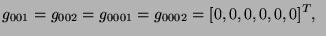 .
The desired nilpotent truncation of
.
The desired nilpotent truncation of
 (valid in the neighborhood of the origin only) can thus be obtained by assuming that
![$\displaystyle g_{001}=g_{002}=g_{0001}=g_{0002}=[0, 0, 0, 0, 0, 0]^T,~$](img374.png) |
|
|
(25) |
as indeed, the values of these brackets evaluated in the neighborhood of the origin are negligibly small. Considering the latter, together with the Lie products which are zero, and the following dependencies among the above Lie products:
 |
|
|
(26) |
which correspond (via evaluation map 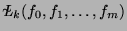 ) to the following symbolic dependencies between the elements of :
 |
|
|
(27) |
for ,  ,
,  , , , , , , ,
  ,
,  , , , , , , , , , , , , a basis for the controllability Lie algebra for system (24)
can thus be defined as:
, , , , , , , , , , , , a basis for the controllability Lie algebra for system (24)
can thus be defined as:
It can be verified that
 is indeed nilpotent if (25) is enforced, and that such nilpotent
corresponds to an STLC system as required.
Additionally, the ordering of this basis satisfies the condition (13), which guarantees that the Wei-Norman equation can be given in the explicit form (14).
The feedback design approach developed in [26] now calls for the computation of an open-loop piece-wise constant control
is indeed nilpotent if (25) is enforced, and that such nilpotent
corresponds to an STLC system as required.
Additionally, the ordering of this basis satisfies the condition (13), which guarantees that the Wei-Norman equation can be given in the explicit form (14).
The feedback design approach developed in [26] now calls for the computation of an open-loop piece-wise constant control
![$\bar{u}:[0,T]\rightarrow \mathbb{R}^3$](img382.png) such that the
such that the  -coordinates for system (24) satisfy
 |
|
|
(28) |
where
 is the value of the -coordinates at time
  and corresponding to the control
 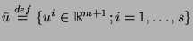 . The set
 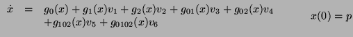 is a set of admissible ``extended controls'' which provide for a monotonic decrease of a given Lyapunov function along the trajectories (originating at a given point
  ) of the extended system to (24) defined as:
The set
 is the reachable set for system (29) in the -coordinates space while employing controls from .
In this context, the idea behind the feedback stabilization algorithm is the following. As has been pointed out in [26], for each satisfying (28) there exists an extended control
is the reachable set for system (29) in the -coordinates space while employing controls from .
In this context, the idea behind the feedback stabilization algorithm is the following. As has been pointed out in [26], for each satisfying (28) there exists an extended control  such that the -coordinates of (24) and (29) match at time ; i.e.
 , where
  are the -coordinates of the flow of the extended system (29). This fact immediately implies that the chosen Lyapunov function decreases (periodically) along the trajectories of the original system (23) (for a precise meaning of ``periodical decrease'' see [26]). To this end, the method in [26] requires the construction of the Wei-Norman equations for systems (24) and (29) where the LTP package yet again comes useful.
Next: Step 2: Calculation of
Up: Example 1: Stabilization of
Previous: Example 1: Stabilization of
Contents
Miguel Attilio Torres-Torriti
2004-05-31
![$\displaystyle [f_0, [f_0, f_1]] =$](img334.png)
![$\displaystyle [f_0, [f_0, f_2]] =$](img337.png)
![$\displaystyle [f_0, [f_0, [f_0, f_1]]] =$](img346.png)
![$\displaystyle [f_0, [f_0, [f_0, f_2]]] =$](img349.png)