Next: Step 1: Construction of
Up: Using LTP: Some Practical
Previous: Example 1: Simplification of
Contents
The usefulness of LTP for practical applications in control of dynamical systems is illustrated by an example of an underactuated rigid body in space for which, after the application of a suitable feedback transformation, the model equations are:
Here  and
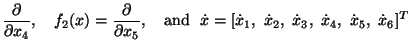
and  are the actuating controls,
  is a scalar constant,
  is the drift vector field, and
  and
and 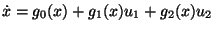 are the input vector fields. For details on the model derivation see, for example [8], and references therein.
The construction of stabilizing feedback control for systems such as (23) can be carried out employing different approaches; one such approach is proposed in [26]. As a point of further interest, it is worth pointing out that model (23) does not lend itself directly to the application of the method in [26] as its controllability Lie algebra is not nilpotent. Its application is made feasible only with the reference to a suitable nilpotent ``approximation'' of the original system; rigorous criteria for obtaining such approximations can be found in [15]. Here, it is demonstrated that even a trivial approximation amounting to a straightforward nilpotent truncation of the controllability Lie algebra for the original system is sufficient for stabilization. The truncation is merely required to preserve controllability of the system. This is justified by the result in [20, Thm. 2]), which shows that the steering error introduced while employing a truncated version of the controllability Lie algebra is a decreasing function of the distance between the initial and target points. It follows that the steering error can be controlled by selecting an adequately small time horizon
are the input vector fields. For details on the model derivation see, for example [8], and references therein.
The construction of stabilizing feedback control for systems such as (23) can be carried out employing different approaches; one such approach is proposed in [26]. As a point of further interest, it is worth pointing out that model (23) does not lend itself directly to the application of the method in [26] as its controllability Lie algebra is not nilpotent. Its application is made feasible only with the reference to a suitable nilpotent ``approximation'' of the original system; rigorous criteria for obtaining such approximations can be found in [15]. Here, it is demonstrated that even a trivial approximation amounting to a straightforward nilpotent truncation of the controllability Lie algebra for the original system is sufficient for stabilization. The truncation is merely required to preserve controllability of the system. This is justified by the result in [20, Thm. 2]), which shows that the steering error introduced while employing a truncated version of the controllability Lie algebra is a decreasing function of the distance between the initial and target points. It follows that the steering error can be controlled by selecting an adequately small time horizon  . Both the degree of nilpotency and the horizon can be selected on a trial and error basis by requesting periodic decrease in a Lyapunov function which is a directly verifiable criterion for the adequacy of the truncation.
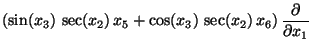
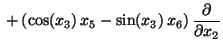
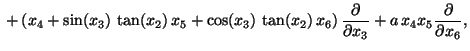
In this context, system (23) is assumed to be approximated by another system of a similar structure
. Both the degree of nilpotency and the horizon can be selected on a trial and error basis by requesting periodic decrease in a Lyapunov function which is a directly verifiable criterion for the adequacy of the truncation.
In this context, system (23) is assumed to be approximated by another system of a similar structure
 |
|
|
(24) |
whose controllability Lie algebra,
 , corresponds to a nilpotent truncation of
 of some finite order. The order of truncation is selected so that the truncated system is STLC (see Theorem 7.3 in [42]). To follow this process, sufficiently many elements in the basis for
need to be known, and one way to proceed is to generate bases for
of some finite order. The order of truncation is selected so that the truncated system is STLC (see Theorem 7.3 in [42]). To follow this process, sufficiently many elements in the basis for
need to be known, and one way to proceed is to generate bases for
 ,
,  in ascending order, to select the smallest
  for which the image of
(under the evaluation map
for which the image of
(under the evaluation map  ) is STLC.
Subsections
Next: Step 1: Construction of
Up: Using LTP: Some Practical
Previous: Example 1: Simplification of
Contents
Miguel Attilio Torres-Torriti
2004-05-31