


Next: Practical Applications of Lie
Up: LIE TOOLS PACKAGE VERSION
Previous: Loading LTP
Contents
Basic Notions and LTP Formalism
This section provides the basic notions and formalism that constitutes a general framework for calculations relevant to the behaviour and properties of dynamical systems. The LTP package relies on this formalism as it is designed to aid analysis and synthesis of systems of basically unlimited Lie algebraic structure. In lay terms, the underlying idea of this formalism is to introduce abstract, but precise algebraic constructs which, under adequately constructed mappings, project directly onto the corresponding constructs acting on manifolds on which the particular systems evolve; see for example Remark 4.1.
To this end, let
 denote a set of indeterminates. For brevity of notation, let
 . Let
. Let  denote the free associative algebra (over
  ) of noncommutative polynomials in the indeterminates
 . Recall that, given a set
  , a free associative algebra on the set over , is an associative algebra over , together with a mapping
 , with the following universal property: for each associative algebra
  and each mapping
 , there exists a unique homomorphism of algebras
 such that
  . Members of have the form of finite linear combinations
 , where the summation is over all possible multi-indices
 , with
 , for
, for  ,
,
 , in which the coefficients
  are real numbers. Here
 , and
, and
 , where, in general,
 as implied by noncommutativity.
Let a Lie product
as implied by noncommutativity.
Let a Lie product ![$[X_i,X_j]$](img29.png) of two indeterminates be defined as the noncommutative polynomial
of two indeterminates be defined as the noncommutative polynomial  . With this definition of the Lie product becomes a Lie algebra. Let
  be the subalgebra of generated by .
The elements of are referred to as Lie polynomials.
Further, let
be the subalgebra of generated by .
The elements of are referred to as Lie polynomials.
Further, let
 denote the Lie algebra of Lie series in
 . The elements of
are formal series of the type
. The elements of
are formal series of the type
 , where
  are coefficients in
  and
and
 . Clearly, any element
 can be written as a formal infinite series
in the indeterminates
, in which
can be written as a formal infinite series
in the indeterminates
, in which  is some monomial in
and
is some monomial in
and
 .
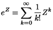
For any element in
the formal power series
.
For any element in
the formal power series
 |
|
|
(1) |
is well defined because
 . Here,
 are infinite series in the indeterminates
obtained by the natural multiplication rule for the
component monomials of
are infinite series in the indeterminates
obtained by the natural multiplication rule for the
component monomials of  ,
,
 , where
  is the juxtaposition (concatenation) of the components of the multi-indices
  and
and  . The set
 is called the
set of exponential Lie series in the indeterminates
.
Note that, due to the antisymmetry property and the Jacobi identity of the Lie product, not all the elements of a Lie algebra
are linearly independent.
A procedure to construct a basis
for any Lie algebra of indeterminates, while taking into account
the dependencies imposed by the antisymmetry and the Jacobi identities,
involves selecting some of the Lie product of
, which can, for example, be carried out in accordance with the rules given below, see [32,36,4].
is called the
set of exponential Lie series in the indeterminates
.
Note that, due to the antisymmetry property and the Jacobi identity of the Lie product, not all the elements of a Lie algebra
are linearly independent.
A procedure to construct a basis
for any Lie algebra of indeterminates, while taking into account
the dependencies imposed by the antisymmetry and the Jacobi identities,
involves selecting some of the Lie product of
, which can, for example, be carried out in accordance with the rules given below, see [32,36,4].
Definition 3.1
- Hall basis (HB). Let

denote the basis for
, and let

be the

-
th element
in this basis. Let the
length (order ) of a Lie product

,

, be defined as
the number of indeterminates in the expansion of
, also given
recursively by:
where
and

are Lie products.
Then a
Hall basis is an ordered set of Lie products

such that:
-
- If
 then
then 
-
![$[B_i, B_j] \in B$](img61.png) if and only if
if and only if
-
 and and
- either
 for some
  or
or
![$B_j=[B_p, B_q]$](img64.png) with
with
 and
and  .
.
The proof that a Hall basis indeed constitutes a basis for the Lie
algebra is found in [14,36].
Remark 3.1
The basis presented above, although already know by P. Hall, was first introduced by M. Hall [
14] and pertains to one of the possible ways in which a basis for
could be constructed. In fact, the above construction was generalized by Scützenberger [
34] by weakening the degree condition 2 in Definition
3.1. Viennot, [
44], further relaxed condition 2 replacing it by:
- 2'.
- If
![$[B_i,B_j]\in B\setminus \bar{X}_m$](img67.png) then
then  and
and ![$B_i<[B_i,B_j]$](img69.png) .
.
The last is so general that it includes the Lyndon basis
and the Širšov basis [
37], which is not the case with the original bases of M. Hall; see [
30,
24,
25] for a comprehensive exposition of different bases constructions.
The choice of the above, rather restrictive, basis construction was deliberate for the purpose of the LTP because it is the one most often used in the engineering literature. Nevertheless, it is worth noting that other bases construction using condition 2' instead of 2 could prove more advantageous in applications for which a particular choice of coordinate system is desirable.
With regard to the algorithmic implementation of the package, a choice of Lyndon basis would possibly offer some advantages. A
Lyndon basis is defined as a set of alphabetically ordered Lyndon words over a given alphabet

(which is defined as a set of letters). A
Lyndon word is any nonempty, finite sequences of letters which precedes all its nontrivial proper right factors in any alphabetically ordered set on
; i.e.

is a Lyndon word if for each nontrivial factorization in terms of sub-words

and

,

, the word
precedes
.
From Theorem 5.1 in [
30] it follows that each element of the Lyndon basis can be uniquely rewritten as an element of a Hall basis satisfying Definition
3.1 with condition 2 replaced by 2'. It is the
rewriting system of [
25] that provides a procedure that allows one to translate any Lyndon word into an element of a Hall basis, thus permitting to use words in place of their corresponding Lie bracket expressions. For example, given the alphabet

, the sequence of Lyndon words: 12, 112, 212, 1213, 1223, 3323, translates, in a one-to-one way, into the following Hall basis elements:
![$[X_1,X_2]$](img76.png)
,
![$[X_1,[X_1,X_2]]$](img77.png)
,
![$[X_2,[X_1,X_2]]$](img78.png)
,
![$[[X_1,X_2],[X_1,X_3]]$](img79.png)
,
![$[[X_1,X_2],[X_2,X_3]]$](img80.png)
,
![$[X_3,[X_3,[X_2,X_3]]]$](img81.png)
in

.
On the one hand, operating on words (character strings) requires less memory, but on the other hand, operations on Lie brackets (binary tree structures) can generally take less processing time than those involving words.
Let
 denote the free nilpotent Lie algebra of
order , i.e. a Lie algebra that can be identified with the quotient
denote the free nilpotent Lie algebra of
order , i.e. a Lie algebra that can be identified with the quotient
 , where
 is the ideal spanned by all elements of the Hall basis of order strictly greater than . Hence,
 can be formed by assuming that all the Lie products in of degree strictly greater than are equal to zero. The above procedure can still be employed to construct bases for
simply by forming all the Lie products that satisfy the above properties and whose length does not exceed .
By the result of Campbell, Baker, and Hausdorff, known as the CBH formula, it follows that
can be formed by assuming that all the Lie products in of degree strictly greater than are equal to zero. The above procedure can still be employed to construct bases for
simply by forming all the Lie products that satisfy the above properties and whose length does not exceed .
By the result of Campbell, Baker, and Hausdorff, known as the CBH formula, it follows that
 is closed under multiplication, and is in fact a group, as it can be verified that
  , for any
 . Moreover, the map
 is a bijection from
onto
.
It follows that for any
is a bijection from
onto
.
It follows that for any
 we can compute a unique
 such that
 |
|
|
(2) |
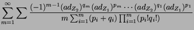
The way to compute  is also delivered by the CBH formula which, in Dynkin's form, is given by [36,39]:
where the inner sum ranges over all  -tuples of pairs of nonnegative integers
  such that
  . In (3), with the exception of the last term, the symbol
  denotes the mapping
![$ad_X:Y\mapsto [X,Y]$](img104.png) for all
for all
 , which is an endomorphism of underlying the adjoint representation of , defined as the mapping
  . With some abuse of notation, the last term in (3) should be understood differently and must be evaluated as follows:
  if
if  ,
,  if
if  , and
, and  if
if  .
It is worth noticing that the group
is not a Lie group because it is infinite dimensional.
As the package is primarily a tool for the analysis of
dynamical systems, it will be applied in the context of groups
of transformations acting on the underlying manifold on which the system
evolves, see [43].
For analytic systems whose accessibility Lie algebras, [32], are finite dimensional, such groups of transformations can be given the structure of Lie groups; see [29]. It is hence helpful to define
.
It is worth noticing that the group
is not a Lie group because it is infinite dimensional.
As the package is primarily a tool for the analysis of
dynamical systems, it will be applied in the context of groups
of transformations acting on the underlying manifold on which the system
evolves, see [43].
For analytic systems whose accessibility Lie algebras, [32], are finite dimensional, such groups of transformations can be given the structure of Lie groups; see [29]. It is hence helpful to define
 , a nilpotent version of
:
, a nilpotent version of
:
 |
|
|
(4) |
The group
is now a Lie group with Lie algebra
, see [43].
For a systematic development it is assumed here that all groups of
transformations act from the right on the underlying manifolds  .
With this notation, for
.
With this notation, for  , the expression
  denotes the value of a group action
  at a point
, [36, p. LG 4.11] or [43, p. 74].
One of the many applications of the LTP package involves the solution of differential equations defined on Lie groups. As will be explained later, the trajectories of these equations relate (through a Lie group homomorphism, see Remark 4.1) to trajectories evolving on
. It is hence convenient that
is equipped with a coordinate system. Such a coordinate system can be constructed in terms of a Hall basis and has the advantage of being global (consisting of a single chart) since
is nilpotent, see [41]. In full rigour, if
at a point
, [36, p. LG 4.11] or [43, p. 74].
One of the many applications of the LTP package involves the solution of differential equations defined on Lie groups. As will be explained later, the trajectories of these equations relate (through a Lie group homomorphism, see Remark 4.1) to trajectories evolving on
. It is hence convenient that
is equipped with a coordinate system. Such a coordinate system can be constructed in terms of a Hall basis and has the advantage of being global (consisting of a single chart) since
is nilpotent, see [41]. In full rigour, if
 is the
  -dimensional Hall basis for a given nilpotent Lie algebra
, then any element
-dimensional Hall basis for a given nilpotent Lie algebra
, then any element  in the Lie group
has the following unique representation, [20]:
in the Lie group
has the following unique representation, [20]:
 |
|
|
(5) |
The map
 establishes
a global diffeomorphism between
and
establishes
a global diffeomorphism between
and  and is thus a global coordinate chart on
. The coordinate system so just introduced falls into the category of Lie-Cartan coordinate systems of the second kind [36,32]. Here, we will refer to it using the name of
and is thus a global coordinate chart on
. The coordinate system so just introduced falls into the category of Lie-Cartan coordinate systems of the second kind [36,32]. Here, we will refer to it using the name of  -coordinates.
Equation (5) can be viewed as a way to represent an arbitrary group
action as a composition of elementary group actions defined in
terms of the elements of the Hall basis of the Lie algebra associated with
the group.
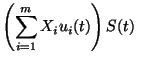
This fact has been exploited by Wei and Norman in the solution of
right-invariant parametric differential equations evolving on
:
-coordinates.
Equation (5) can be viewed as a way to represent an arbitrary group
action as a composition of elementary group actions defined in
terms of the elements of the Hall basis of the Lie algebra associated with
the group.
This fact has been exploited by Wei and Norman in the solution of
right-invariant parametric differential equations evolving on
:
where  (finite),
  are indeterminate operators independent of
 that generate
under
the commutator product
that generate
under
the commutator product
![$[X_i,X_j]=X_jX_i-X_iX_j$](img133.png) , and
, and  are
scalar functions of . Here, as
are
scalar functions of . Here, as
 ,
,  evolves
on
.
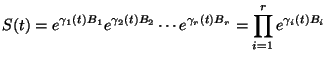
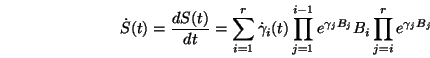
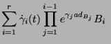
Therefore, the solution to (6) is given by the product of exponentials:
evolves
on
.
Therefore, the solution to (6) is given by the product of exponentials:
 |
|
|
(7) |
where
is the Hall basis for the Lie algebra
, and the  are scalar functions of time,
see [41,45]. Without the loss of generality, it may be assumed
that
are scalar functions of time,
see [41,45]. Without the loss of generality, it may be assumed
that  , for
, for  .
.
Remark 3.2
The representation (
7) of the solution to equation (
6) is not unique. Alternatively, the solution to (
6) can be represented using the Lie-Cartan coordinates of the first kind, i.e. it is possible to write
where

,
, are the ``coordinates'' of such a solution; see [
22].
Remark 3.3
For an arbitrary set of indeterminates
the Lie algebra
is really infinite dimensional. A unique solution of (
6), however, still exists for every Lebesgue integrable control function
![$u\stackrel{def}{=}[u_1,\ldots,u_m]$](img144.png)
defined on a finite interval
![$[0,T]$](img145.png)
. This solution is known to evolve on
, see [
40, Prop. 3.1]. Furthermore, the solution of (
6) can be written in terms of a formal power series in the indeterminates
, denoted by

, and known as the Chen-Fliess series, see [
12, Theorem III.2, p. 22]. The coefficients in
are iterated integrals of the control functions
and for any
,

, where

denotes the Chen-Fliess series with coefficients evaluated over
![$[0,t]$](img150.png)
.
It has been shown in [
41] that the expression of the the solution of (
6) in the form of a Chen-Fliess series
is equivalent to the expression in the form of a product of exponentials, i.e. for any given control function
, there exist functions
![$\gamma_{i}:[0,T]\rightarrow \mathbb{R}$](img152.png)
,
such that (
7) is valid with the product performed over all members of the P. Hall basis
for
.
A particularly convenient formalism based on chronological algebras introduced for nonstationary vector fields has been introduced in [
1] and permits to re-write the Chen-Fliess series in a very compact and symbolically tractable form, in which the iterated integrals are re-expressed in terms of the
chronological product operations, see [
18,
17]. The chronological calculus has also been shown useful in the calculation of the logarithm of the Chen-Fliess series, see [
31]; however, the expressions derived there, although relatively simple, provide a series expansion of this logarithm which may contain linearly dependent terms.
The -coordinates in (7) are shown to satisfy a set of nonlinear differential equations as is implied by the following derivation, see also [45,32].
Differentiating (7) yields,
 |
(8) |
Multiplying both sides of (8) by  from the right
and using the exponential formula (see [43, p. 40]):
from the right
and using the exponential formula (see [43, p. 40]):
yields,
| |
 |
 |
(11) |
with  for
for
 , as satisfies (6).
Equating the coefficients on both sides of the last equality gives:
, as satisfies (6).
Equating the coefficients on both sides of the last equality gives:
where the
 are analytic functions of the 's.
Clearly,
are analytic functions of the 's.
Clearly,  since
since 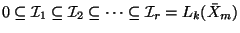 .
It is worth noting that there exists a chain of ideals
.
It is worth noting that there exists a chain of ideals
 where each
  is exactly of dimension
  . The order of the elements in the Hall basis
 is such that is the ideal is generated by
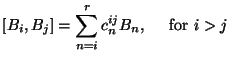 , which implies that the multiplication table for
satisfies:
, which implies that the multiplication table for
satisfies:
![$\displaystyle [B_i,B_j]=\sum_{n=i}^{r} c^{ij}_n B_n,\hspace{5mm}\textrm{for}\ i>j~$](img176.png) |
|
|
(13) |
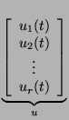
It can be shown, see [45], that such a multiplication table implies that 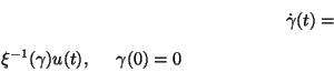 is lower triangular and invertible for all . Hence, (12) yields the system of differential equations for the computation of the -coordinates in explicit form:
 |
(14) |
Equation (14) will be referred to as the Wei-Norman equation.
Its solution delivers of (7) which solves (6). The explicit formulæfor the solution of (14), in terms of iterated integrals, are also given in [41]; see also [18, Thm. 4.10, p. 297].
Next: Practical Applications of Lie
Up: LIE TOOLS PACKAGE VERSION
Previous: Loading LTP
Contents
Miguel Attilio Torres-Torriti
2004-05-31
![\begin{eqnarray*}
l(X_i)&=&1\hspace{2cm} i=1,\ldots,m\\
l([G,H])&=&l(G)+l(H)
\end{eqnarray*}](img55.png)

![$\displaystyle \underbrace{
\left [\begin{array}{c}u_1(t)\\ u_2(t)\\ \vdots\\ u_r(t)\end{array}\right ]}_{u}$](img166.png)