


Next: Function Reference
Up: Using LTP: Some Practical
Previous: Step 2: Calculation of
Contents
The aim here is to construct a finite dimensional realization of a nonlinear filter for the stochastic system described by (see [28,19]):
where  and
and  are independent Brownian motions. As suggested in [5] such a realization can be derived by applying Lie algebra techniques to the DMZ equation for the unnormalized conditional density
  , given the observation process
 for system (29). The DMZ equation here is
where the differential operators
 are defined by the following expressions on their common invariant domain
  which is dense in
 (see [28]):
It will first be shown that the estimation Lie algebra
 for the above problem is finite dimensional and solvable. Then, the solution of the Cauchy problem for any given
 , representing the conditional density of
 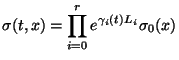 , can be written in the form of a product of exponentials, see [23]:
 |
|
|
(30) |
where  ,
,  is a basis for the Lie algebra
  . The exponential
 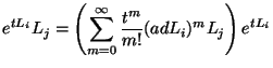 represents here a strongly continuous one-parameter semi-group operator defined on a Banach space
and corresponding to the infinitesimal generator . The last representation is only valid if the Baker-Campbell-Hausdorff-Zassenhaus formula:
represents here a strongly continuous one-parameter semi-group operator defined on a Banach space
and corresponding to the infinitesimal generator . The last representation is only valid if the Baker-Campbell-Hausdorff-Zassenhaus formula:
 |
|
|
(31) |
holds for all the ,  ,
,
 . As pointed out in [28] the validity of (31) is guaranteed if there exists a common, dense (in
), invariant under , set of analytic vectors for the estimation Lie algebra spanned by , . Such a set can be constructed as the linear span of eigenvectors of the operator
. As pointed out in [28] the validity of (31) is guaranteed if there exists a common, dense (in
), invariant under , set of analytic vectors for the estimation Lie algebra spanned by , . Such a set can be constructed as the linear span of eigenvectors of the operator 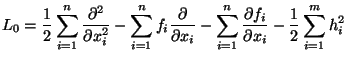 .
To check the solvability of , the differential operators and
.
To check the solvability of , the differential operators and 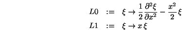 are first defined in Maple as follows:
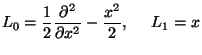
> L0:=xi->(1/2)*diff(xi,x$2)-(1/2)*x^2*xi;
  L1:=xi->x*xi;
A basis for the Lie algebra of operators  is obtained by considering a free nilpotent Lie algebra
  , where
  is a sufficiently high order and calculating its P. Hall basis. For example, for
  , the P. Hall basis for
 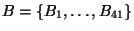 ,
,
 counts 41 elements and is constructed by invoking B:=phb(2,7). In this process, the package also delivers explicit bracket expressions for the basis elements in
  which are omitted here for reason of brevity. Identifying
 ,
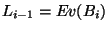
,  , the basis elements in can thus be evaluated next by executing the LTP function calcLBdiffop(B[i],B[1..2],[L0,L1],[x]), for i
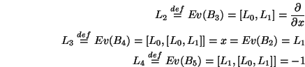 , yielding:
It can further be verified that the application of the evaluation map  to the remaining brackets in the basis B reveals several linear dependencies between
,
to the remaining brackets in the basis B reveals several linear dependencies between
,  :
:
 ,
,
 ,
,
 , and
, and 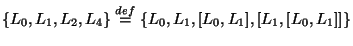 , for the remaining Lie products. From this calculation it follows that a basis for can be defined as
![$\{L_0,L_1,L_2,L_4\}\stackrel{def}{=}\{L_0,L_1,[L_0,L_1],[L_1,[L_0,L_1]]\}$](img443.png) . These calculations also show that the derived Lie algebra
. These calculations also show that the derived Lie algebra ![$[L_E,L_E]$](img444.png) is spanned by
is spanned by  and
and 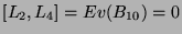 , and is nilpotent because
![$[L_2,L_4]=Ev(B_{10})=0$](img447.png) . Hence, the Lie algebra is solvable, by Corollary 5.3 in [36].
The representation (30) now becomes:
. Hence, the Lie algebra is solvable, by Corollary 5.3 in [36].
The representation (30) now becomes:
 |
|
|
(32) |
is hence valid globally, see [45], and the functions  ,
,  can be computed by quadrature of the Wei-Norman equations. The analytic expression for the Wei-Norman equations can be derived by executing the sequence of commands:
r:=4; # Basis dimension.
max_bracket_order:=6; # Degree of nilpotency minus one.
wn:=wner(r,max_bracke_order,BB,B,[SR]):
wnfe:=wnde(wn,r,{},BB,{}):
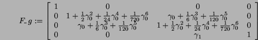
F_g:=eval(wnfe[1]):
The symbol [SR] is a Maple list containing the dependencies between the members of the basis after application of the evaluation map as derived above. The symbol F_g assumes value of the matrix 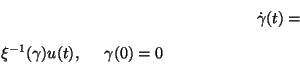 of equation (12) and is here:
The entries  and
and  of F_g can be clearly be recognized as the first few terms in the Taylor series expansion for
  . Similarly, the entries
  and
and  are recognized as the first few terms of the Taylor series for
  . Now, it can be verified that if the above calculations are repeated using a Hall basis of order
  , then the entries of F_g will contain higher order terms of these Taylor series. Thus, by induction, it can be shown that these entries truly are the and functions, so that the Wei-Norman equations for (32) in the form (14) are given by:
where
![$u=[1\ dy(t)\ 0\ 0]^T$](img459.png) .
The solution of these Wei-Norman equations constitutes the joint-sufficient statistics for the linear filtering problem of (29). Now, Mehler's formula (see [28]) allows to obtain the explicit expression for the one parameter semi-group
.
The solution of these Wei-Norman equations constitutes the joint-sufficient statistics for the linear filtering problem of (29). Now, Mehler's formula (see [28]) allows to obtain the explicit expression for the one parameter semi-group
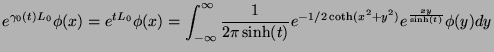 in the form of an integral operator as follows:
 |
|
|
(33) |
for any
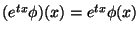 .
Since
.
Since
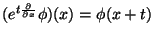 and
and
 , then, finally, (32) and (33) combine into:
which is an explicit formula for the nonlinear filter for (29).
Next: Function Reference
Up: Using LTP: Some Practical
Previous: Step 2: Calculation of
Contents
Miguel Attilio Torres-Torriti
2004-05-31