Figure 7.1. An implementation of the Karplus-Strong algorithm (J. Clark).
The reason for the relative success of physical modeling in synthesizing strings and woodwinds is that the sound generation process in these instruments can be described as an excitation of a transmission line or waveguide. The mathematical equations describing such structures are rather simple (wave equations) and straightforward to implement computationally.
In a waveguide or transmission line model, the vibrating portions of an acoustic instrument are broken up into short segments. In each of these segments the incoming wave is partially transmitted to the next segment, and partially reflected back to the previous segment. A portion of the input is also lost (neither reflected or transmitted) as heat. In more complex models, a portion of the input can also be stored, typically in the elastic material making up the instrument. These complex models can be very nonlinear and difficult to control. They are also very challenging to implement computationally in a stable manner.
Another important aspect of the waveguide segments is the propagation delay time for the input to make its way to the next segment. This delay time can also vary with the frequency of the signal. Frequency dependent delays result in spectral dispersion, which can be useful in modeling complex sounds such as cymbals.
The relative amounts of input that are transmitted, reflected, lost, or stored in a waveguide section, along with the delay time of the section, are the parameters that determine the sound of the instrument. These parameters can also vary with the frequency of the input. For example, more high frequency energy can be lost than low frequency energy, resulting in a sound that progressively gets duller. By piecing together a string of such sections, with appropriate values of the parameters, we can get a sound which closely approximates that of a given acoustic instrument.
One can combine the averaging process with the delayline readout and re-writing process. To do this, the delayline can be continually read-out and re-written, one sample at a time. The output of the delayline can be passed into a lowpass filter (which does the averaging) and the output of the filter fed to the input of the delayline.
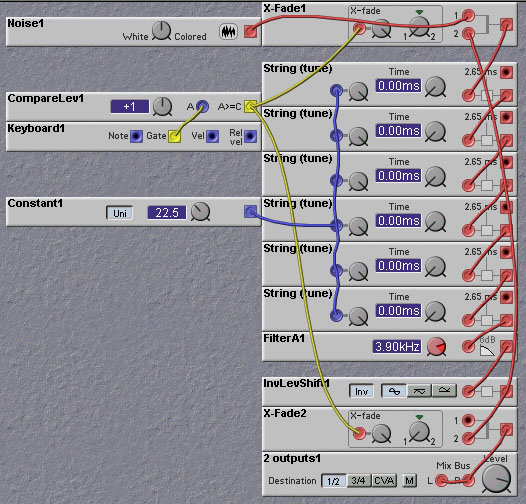
Implementing the Karplus-Strong algorithm on the Nord Modular is simple. Connect a crossfade module in the feedbackloop of the delay. Switch the crossfade with a short pulse from the logic pulse module filling the delay with some sound, which might be noise, or your voice. Then you hear this little 'soundsample' play a frequency that is controllable by the delaytime. To attenuate the input to the delay line in a frequency dependent manner a simple 6dB fixed lowpass filter module can be used. This filter's response is very similar to the 'summing and divide by two' method, but is more flexible, as by varying the frequency of the filter one can obtain a longer or shorter decay time.
Such a simple implementation of the Karplus-Strong algorithm is shown in the figure below:
There are some improvements possible on the algorithm, but sadly not on the Nord Modular. For instance, by having a table (looped delayline) of fixed length and separating the averaging routine and the table readout routine reading out in variable interpolated steps the decay is no longer frequency dependant but can be varied by the speed that the table is averaged. Also there is better control over the frequency that is hard to control on the Nord Modular. By using two tables and 'pre'-filling one table and switch to the new table on the next gatepulse, the averaging can start immediately without having to wait to fill the table. That definitely improves the attack with longer tables and non-noise audio-input. It can sound much better that it does now. When the averaging goes with less speed a nice very lifelike and an `acoustic' soft phasing is introduced in the sound.
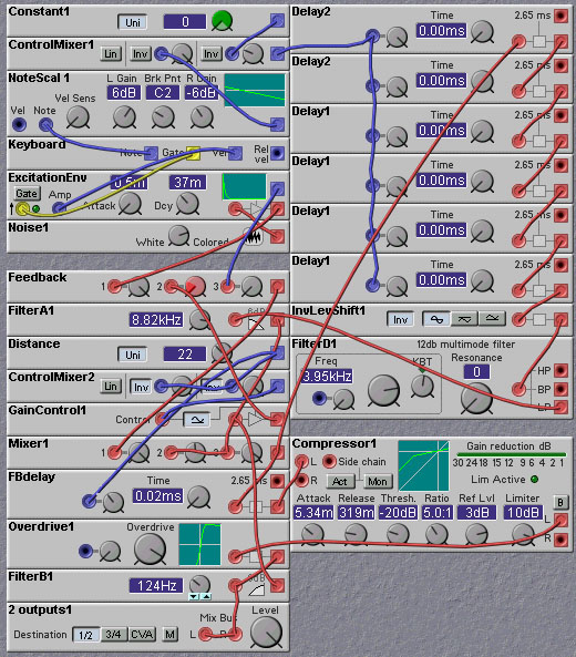
Sean Costello points out that one can simulate guitar feedback with a simple Karplus-Strong algorithm (this was described in a CMJ article in the early 90's). To do this, feed the output of the Karplus-Strong delay lines (one for each of the 6 strings) into a nonlinear shaping function that simulates an overdriven amplifier and fuzzbox. You can also compress the output to provide sustain. Feed a portion of the output into another delay line, to simulate the distance from the amplifier to the "strings". This delay line then feeds back into the Karplus-Strong delay lines. By controlling the amount of the output fed into the delay line, and the length of the delay line, you can control the intensity and pitch of the feedback note. A Nord Modular patch that implements this feedback guitar is shown below. In this patch knob 3 controls the "distance" between the simulated amp/speaker and the string. Changing the distance changes the feedback delay time as well as changing the amount of feedback.
The first factor to consider is that the delaytime of the Nord Modular
delaytimes is a linear function of the delay control input. But the
pitch of the resulting sound is inversely proportional to the
delaytime. Thus, we need some way of computing the reciprocal of the
pitch control value (e.g. from the keyboard module). Clavia does not
(yet) supply an inversion module. Fortunately, there is a module that
can be coerced into doing what we want. Richard Thibert, in his
"physicflute" patch,
discovered that a NoteVelScaler module can be
used to implement the required reciprocal computation. More precisely,
it computes the reciprocal of the exponential of the note number,
which is actually what we want, since the pitch is exponentially
related to the note number.
This approach to tuning is illustrated in the following Nord Modular
patch, made by Rob Hordijk:
Note that the gain of the NoteVelScaler has been set to -6dB/octave.
This value gives the desired reciprocal operation. A short pulse of
noise is inserted into the delay line whenever a key is pressed. This
simulates the plucking of a string. The feedback level of the
delayline back into itself can be adjusted. This sets the decay rate
of the waveform. If the feedback is too high, the loop can become
unstable. The filter in the loop controls the relative rate at which
high and low frequencies become attenuated. Adjusting the cutoff
frequency of this filter controls the `brightness' of the sound.
Another, more subtle, factor influencing the tuning of physical models
are the computational delays inherent in the various operations going
on. For example, the filters that are used to provide the frequency
dependent attenuations generate some delay. Since the filter delay is
not influenced by the delayline delay time (since they are independent
modules) the result will be a fixed shift in delay, causing a detuning
of the sound, especially at high frequencies, where this fixed filter
delay is relatively larger in comparison to the delay line delay time.
This high frequency detuning can be compensated for somewhat by adding
in an extra pitch-dependent delay time (what in the older days was
called 'high frequency-tracking') or by slightly reducing the control
value being sent to the delaylines by small amounts at high pitch
values. In the above patch this is accomplished by adding in a
note-value dependant `constant' to the tuning signal coming from the
NoteVelScaler module.
Another issue to consider when trying to tune delay lines is whether
the delayline has a variable length, but constant time step, or a
constant length with variable time step. Think of modeling a
guitar. You can increase the pitch either by tightening the string
(which increases the propagation speed) or by making the string
shorter. When working with a variable length/fixed step delayline the
decay of the plucked string gets shorter in proportion to the pitch of
the sound. But in a guitar the high strings have more or less the same
decaytime as the low strings. So for KarplusStrong patches it's much
better to work with a fixed length / variable step delayline. Then you
can have the whole frequency range from very, very low to over 20kHz
within a 256 sample delayline! It also gives the possibility to 'eat'
the samples up with a steprate independent of the frequency!
Unfortunately, this is not an option with the Nord Modular, as the
only delayline modules that are available are of the variable length
fixed step size type.
Finally, one should consider the total range of pitches that are
available to physically modeled instruments on the Nord Modular. The
maximum frequency depends on the minimum delay of a string of
delay-lines. This is not a problem, as one can readily make an
instrument that can produce supersonic pitches. The major difficulty
arises when trying to achieve low pitches. The lower the required
pitch the longer the required delay line. Because of the amount of
memory and DSP resources used by the delay line module, one can only
string together at most 6 delay lines. One trick of waveguide
synthesis is to make sure that the reflected portion of the waveguide
segment has an inverted sign relative to the input. This will
effectively drop the pitch by one octave. This trick also cancels
'DC' components that could build up while feeding back, if the average
DC of the input signal would be different to zero level (which would
eventually force the delayline to overflow).
The first thing that people notice about the delay line modules is
that they use a relatively large proportion of the systems's DSP
cycles and memory. The reason for the high memory usage is basically
that the Nord Modular has very limited memory available resources, so
it doesn't take much to use it all up.
The high DSP load for the delay lines may appear to be puzzling at
first, especially when you consider that to compute a delay line
should only require one memory read, one memory write, and one pointer
increment. But the Nord Modular delay line module has the ability to
have delay times that are non-integer (i.e. fractional) multiples of
the sampling period. In order to achieve this high resolution,
interpolation is performed, which involves filtering of the data
stored in the delay line. This filtering is what consumes most of the
DSP cycles. This DSP usage is a good price to pay for the ability to
accurately tune the delay lines. If interpolation was not done, then
it would not be possible to have a properly tuned physically modeled
instrument.
The actual resolution of the delaytime in the Nord Modular is very
high. Although Clavia has not released any figures on this, it is
estimated that the resolution is 2^19 steps in 64 control units, or
5.05 nsec over the 0-2.65 msec range.
One of the drawbacks of using interpolation to obtain high delaytime
resolution is that the interpolation always attenuates the signal in a
frequency dependent manner. If you apply a Gaussian Blur (a form of
weighted interpolation) to an image, the sharp edges and details --
the high frequencies -- get lost. The same takes place if you
interpolate an audio signal. After a single pass, the loss of high
frequencies is not that noticable, but if you repeatedly pass the
signal through the process of interpolation, the signal is attenuated,
and eventually decays down to zero. In any delay line, there is
always this trade-off between accurate delay time (giving acurate
pitch in a physical modelling waveguide configuration) and accurate
frequency response.
Making a physically modeled instrument consists of connecting a series
of these waveguide sections. Note that each waveguide section has two
signals going into it, and two signals going out. These two sets of
signals model the waves travelling in one direction, and the waves
travelling in the opposite direction. Each section contains two
summers, six attenuators, and two delay lines. The delay lines models
the time it takes for the wave to propagate from one end of the
section to the other, in either direction. The attenuators with values
g and -g model the losses that may occur in the waveguide. For
example, energy can be lost in a vibrating string by acoustic
radiation, or by heating the surrounding air. These losses can be
frequency dependent, and typically losses are greater for high
frequencies than for low frequencies. In this case the attenuators
would be implemented with lowpass filters. The other attenuators
(with values of r, -r, 1+r and 1-r) model the scattering of the signal
at the junction between two sections - part of the signal is
transmitted across the junction, while the rest is reflected back in
the opposite direction. These attenuations are also usually frequency
dependant, that is, the relative proportion, r, of signal that is
reflected at a junction depends on frequency. Thus these attenuators
are often implemented with filters. Typically the reflection
coefficient r has a lowpass characteristic (and therefore 1-r has a
highpass characteristic), modeling the usual physical situation that
high frequencies are transmitted preferentially, and low frequencies
are reflected preferentially. Different sections can have different
characteristics. This change in characteristic from section to
section can model physical systems that have changing geometry, such
as a woodwind with a non-constant bore diameter. A termination of the
waveguide can also be modeled in this way, by setting the reflection
coefficient to r=1, thereby causing all of the energy to be reflected.
In some instruments, such as brass instruments, sound can be radiated
from the termination point. In this case r is not set to one, but is
set to a lowpass characteristic, with the low frequency response equal
to one. The transmitted energy will have a high pass characteristic
and will form the output signal.
The reflection coefficients for the intermediate waveguide sections
are set to zero. This models the fact that the strings are uniform
along their length, and do not have any discontinuities that would
cause reflections. The only reflections occur at the termination
points of the string. The loss coefficients k are taken to have a
lowpass characteristic, modeling the loss of high frequency energy as
waves propagate along the string.
The string is set into motion by creating an initial displacement
somewhere (anywhere) along the string. This models a percussive
`striking' of the string.
The output can be taken from any point along the modeled string, and
is obtained by summing together the forward and backward waveforms (as
these together determine the string displacement). The overall model
for the string is shown in part A) of the figure below.
This model is more complicated than it needs to be, however. The
circuit is completely linear in the mathematical sense. This means
that we can combine all of the delaylines into one
delayline. Similarly, we can combine all of the lowpass filters into a
single lowpass filter, which models the overall frequency dependent
losses. We can even combine the inverters, which, since their effect
cancels, means that we can remove them. Doing these modifications
results in a much simpler model, shown in part C) of the figure above.
This simplified model is implemented in the following patch:
Notice the similarity between this patch and the Karplus-Strong
patches shown earlier. The only real difference is in the way in which
the string is excited, or struck. In the Karplus-Strong patch, white
noise was used to initialize the delayline (and hence the initial
string displacement). In the digital waveguide patch, the initial
displacement is an impulse at one end of the string. The impulse could
be modeled as occuring anywhere along the strong. But to do this, one
needs to break the waveguide into two parts - one before and one after
the point of the impulse. Thus it will be a somewhat more complex
model than the simple one shown above. Using an impulsive (in space,
along the string) excitation is not very realistic. In a real guitar,
for example, the string is excited by pulling it sideways at the
plucking point. Thus the initial waveform is a smooth displacement
along the length of the string. To accurately model such an excitation
we would need a large number of waveguide sections, each with a small
delay, and relatively little frequency dependance in the transmission
and reflection amounts.
Coupled Strings
In most stringed instruments there is more than one string
present. These strings do not oscillate independently of each other,
but interact. The interact takes place through transmission of some of
the energy of each vibrating string to the other strings. This
transmission takes place through the body of the instrument that the
strings are attached to. In a guitar, for example, most of this
coupling takes place at the bridge, where the strings are fixed in
close proximity. If the bridge was infinitely stiff there would be no
coupling, but if it is somewhat non-rigid, part of the vibrational
energy of a string will go into creating a small vibration of the
bridge, which will then be transferred in part to the other strings.
Coupling between strings can be implemented in a digital waveguide
model as shown in the following diagram:
A non-rigid bridge will introduce losses, and one can eliminate the
loss filters in the individual string models, thereby simplifying the
design. Only one filter is needed, that modeling the bridge. A Nord
Modular patch implementing this simplified model is given in the
following figure.
The excitation process is more complicated in woodwinds
than in strings. One does not `pluck' a clarinet, one blows into
it. The key aspect of the excitation of a clarinet is the reed. The
reed acts as a nonlinearity, affecting the flow of air into the bore,
as well as the reflection of the pressure wave at the mouth end. In
simple terms, as a pressure differential across the reed is built up
by blowing into the mouthpiece, the amount of reflected energy
increases. Further pressure increases, however, begin to close the
reed, and the amount of reflected energy begins to drop, going to zero
once the reed closes. This nonlinearity, driven by the pressure
provided by the player, provides amplification or gain in the loop
formed by the outgoing and reflected pressure waves. If the gain is
high enough, oscillation can occur. This oscillation is what provides
the basic tone of the clarinet. The frequency of oscillation depends
on the total delay time of the loop. Unlike a string, the nonlinearity
at the mouth end of the clarinet causes the creation of harmonics,
giving the characteristic square wave tone of the clarinet. In a
physical model on a computer or a Nord Modular, one can increase the
gain of the nonlinearity, and create different regimes, including
chaotic ones, where the frequency components created by the
nonlinearity are inharmonic and noisy.
In the Nord Modular it is difficult to implement a precise model of
the nonlinearity of the clarinet excitation, but one can easily
implement an approximation. In the patch shown below we use the WaveWrapper
module to provide an approximation to a cubic nonlinearity, which is
known to work well in generating oscillations. We use the Shaper
module to round off the corners of the WaveWrapper function a bit. The
effect of the mouth pressure is faked somewhat as compared with what
occurs in a real clarinet. In this patch the breath input (modeled as
the output of the Envelope Generator module) is used to vary the gain
of the nonlinearity. If the gain is too low, no oscillation will
occur. In real clarinets the effect of the mouth pressure is to shift
the nonlinearity along a 45 degree line. This is hard to implement
with the Nord Modular, so we will stick with the simple approximation.
You should play around with this patch a bit, and especially explore
the effect of changing the gain of the nonlinearity by adjusting the
level of the third input to the Mixer module. It is quite easy to get
chaotic sounds. A schematic diagram of this model is shown in the next
figure, and the Nord Modular is shown in the figure following it.
Tone-hole Modelling
In the above patch, while it sounds like a clarinet, we cheated in
modeling the tuning. The pitch of a real clarinet isn't changed by
changing the length of the instrument bore! Rather, pitch changes are
obtained by opening and closing `tone-holes' in the instrument body.
To a first approximation, one can consider the sound emitted by the
instrument as coming entirely from the first open tonehole (nearest to
the mouthpiece). The tonehole will transmit a portion of the energy
and reflect the rest. Typically high frequency energy is transmitted
and the low frequencies are reflected. Thus we can implement the
tonehole as a pair of filters, a lowpass for the reflection and a
highpass for the transmission. To reduce computational load, we can
implement the highpass filter simply by subtracting the lowpass output
from its input. To reduce computation even further we can model the
tonehole just as a switch. When it is closed it transmits all of the
energy, and reflects nothing, and when it is open it reflects all of
the energy and transmits nothing. The losses can be lumped together in
a single loop lowpass filter. The energy transmitted by each tonehole
are summed together, although in the simple model being used only one
tonehole at a time (the one closest to the excitation) will have any
output. In a multiple tonehole instrument we can use switches to
select which tonehole the sound will be reflected from/transmitted
through. This simple approach is used in the patch shown in the figure
below.
In this patch NoteDetect modules are used to select which toneholes are
open. This is opposite to what you would normally do with your
fingers when playing an instrument with toneholes, i.e. press down
your fingers to close the tonehole. The reason for doing it this way
in the patch is to allow MIDI'ed wind-controllers to drive the
patch. These controllers convert the closures on the instrument into
corresponding MIDI note values. They do not transmit tone-hole
closures. If you want to change the patch so that key-downs close the
toneholes instead of opening them, you simply need to swap the outputs
of each of the Pan modules in the patch.
Note that the outputs of the NoteDetect are passed through Smoothing
modules before being fed into the Pan control inputs. This is to
eliminate the objectionable elastic click which would otherwise occur
when closing one tonehole and opening another. This click is caused by
discontinuities in the audio DelayLine modules. Going from one note to
another requires a re-configuration of the instrument's overall delay
line structure. If one plays in a legato style, and moves from a low
pitched note to a higher pitch, there will be little problem. Playing
in a staccato fashion, or moving from a high pitch to a lower requires
switching in extra delay line sections to the currently active ones.
The currently active section has the ongoing wave passing through it,
whereas the new sections will just have zeros in them. Thus there will
be a significant discontinuity in the wave passing through the
reconfigured delay line section. This discontinuity will be quickly
smoothed out but it is enough to give a noticeable
transient. Transients such as these DO occur in real instruments, but
they are of a less objectionable nature than in our simple model. We
will have to do a better job of modelling the tonehole-bore interfaces
to obtain more natural transitions between notes.
Slide-Flute
Perry Cook has devised many physical models of
musical instruments. One of them is the "Slide-Flute", which he described
in the following conference paper:
Cook, P., "A Meta-Wind-Instrument Physical Model, and a Meta-Controller
for Real Time Performance Control", Proceedings of the ICMC, 1992.
The slide flute model consists of two delay lines, one to model the
flute's bore and the other to model the embouchure (the opening into
which the player blows to sound the flute). The length of the flute
bore delay is twice that of the embouchure delay line. A Nord Modular
patch implementing this model is shown below. In this patch a
wave-wrapper module is used to simulate the nonlinearity of the
excitation and the interaction between energy bouncing back from the
end of the flute bore with incoming breath pressure. The output from
the bore delay line is fed back into the system in two places. The
jet delay knob simulates changing the angle with which the player
blows into the flute - thereby allowing overblowing techniques. In
this patch the jet delay is also controlled by the mod wheel.
All-Pass Filter Delays
There are other ways to obtain delays with the Nord Modular than the
delay module. For example, delays in analog and digital signal processing
systems are often obtained with all-pass filters. An all-pass filter
is a filter that doesn't change the spectrum of the input, that is, the
frequency response of the filter is flat. What is the use of this, you ask?
Well, while the frequency response of the filter may be flat, its phase
response is not. If the phase shift imposed by the filter changes linearly
with frequency, the effect will be to cause a constant delay. We can implement
an all-pass filter in the Nord Modular by combining a low-pass filter and
a high-pass filter in parallel. In fact, we can use the multi-mode
"D"-filter module and just sum its HP and LP outputs.
The resulting phase is not linear, however. The delay is greatest near the
cutoff frequency of the HP and LP filters. The frequency-dependent delay
will cause 'dispersion', which may distort the sound if harmonics exist. For
a pure sinusoidal waveform, there should be no distortion.
An example of
this approach is given in the slide flute
patch shown below. It is more difficult with this patch to ensure that
the flute bore delay is twice that of the embouchure delay, so the sound
is not as good as the previous slide flute patch, but it uses about 25%
less DSP power.
7.3 Tuning of Delay Lines
The pitch of acoustic sounds generated with digital waveguide models
depends mainly on the delaytime of the waveguide segments. Thus,
tuning the instrument involves setting the proper delaytimes. On the
Nord Modular, this is a bit trickier than it may seem at first, due to
a number of factors.
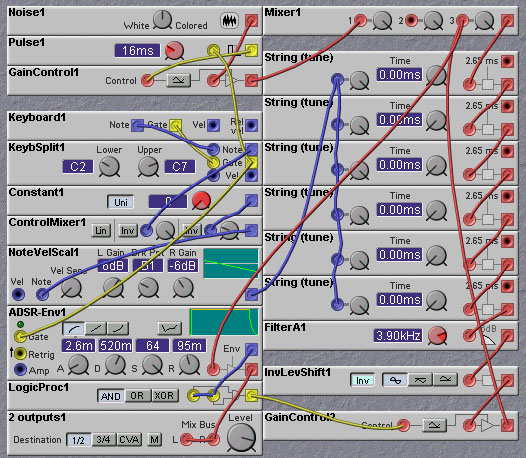
Figure 7.3. Tuning of a Karplus-Strong delay-line using the
NoteVelScaler module (R. Hordijk).
7.4 Delay Line Details
The delay line modules provided by Clavia in the Nord Modular are the
fundamental components of any physically modeled instrument, so it is
useful to know a little about their characteristics.
7.5 Physical Modeling with Digital Waveguides
The transmission lines or waveguides that make up a physically
modeled acoustic instrument are easily implemented with digital filter
structures. These have been termed digital waveguides. The
typical form of a digital waveguide is shown in the figure below.
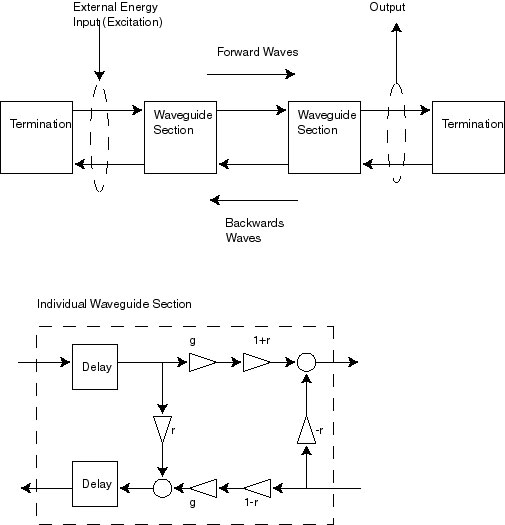
Figure 7.4. Digital waveguides consist of digital filter
implementations of lumped waveguide sections.
7.6 String Modeling
Perhaps the most straightforward instrument to model with a digital
waveguide is a string. A string is modeled as a set of waveguide
sections connecting two special `termination' waveguide sections. The
termination sections model the rigid connections at either ends of the
string. The model for these terminations is quite simple - just an
inverter. This inverter implements the inversion of the wave that
occurs during reflection at the rigid termination. This inversion
occurs because at, the end point, the forward and reflected waves must
sum to zero in order to keep the end point from moving. This is
equivalent to setting the reflection coefficient of the terminating
waveguide sections to r=-1.
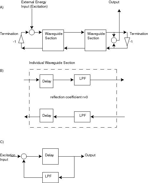
Figure 7.5. Digital waveguide model of a vibrating string. A) A
multiple-section model. The inverters at either end model the rigid
terminations of the string, which requires that the amplitudes of the
forward and backward going waves at these terminations sum to zero. B)
The individual waveguide sections consist of two delay lines and two
lowpass filters. The reflection coefficient is set to zero, modeling
the uniformity of the string.
C)
A simplified model, using the linearity of the network to combine elements.
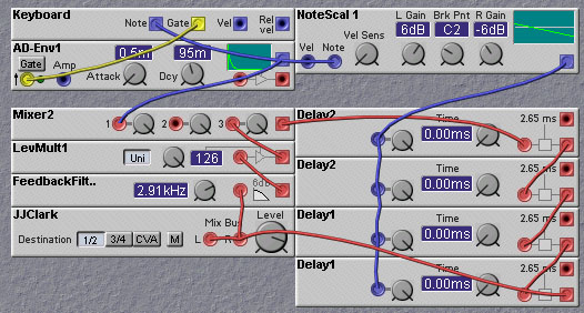
Figure 7.6. A Nord modular patch implementing a lumped digital
waveguide model of a vibrating string (J. Clark).
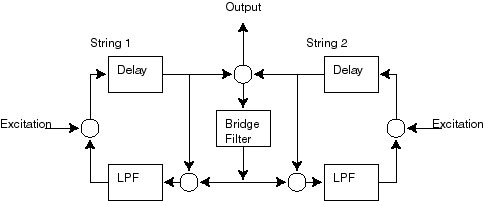
Figure 7.7. Physical model of two coupled vibrating strings.
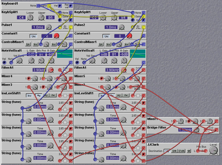
Figure 7.8. A Nord modular patch implementing coupled vibrating
strings (J. Clark).
7.7 Woodwind Modeling
Woodwinds are also suitable candidates for physical modelling. As with
strings, waveguide sections can be used to model the propagation of
waves up and down the tube of the instrument. Woodwinds are somewhat
more complicated to model than strings, because the bore of the
woodwind can change along its length, whereas the string has a more or
less constant thickness along its length. In addition, the bore can
contain holes which also need to be modeled. That being said, a simple
woodwind model looks very much like a string model. We can assume that
the instrument bore has a constant diameter (as in a clarinet), and
has no holes, except at the end. Clearly, the lack of holes is not a
realistic assumption, as it doesn't seem to give us anyway of changing
the pitch! We can cheat, however, and vary the pitch by changing the
delay time of the waveguide section delays, much as is effectively
done in instruments such as the kazoo or trombone.
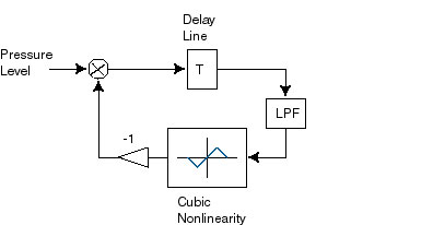
Figure 7.9. A simple digital waveguide model of a clarinet.
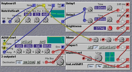
Figure 7.10. A Nord Modular implementation of the simple clarinet
model (J. Clark).
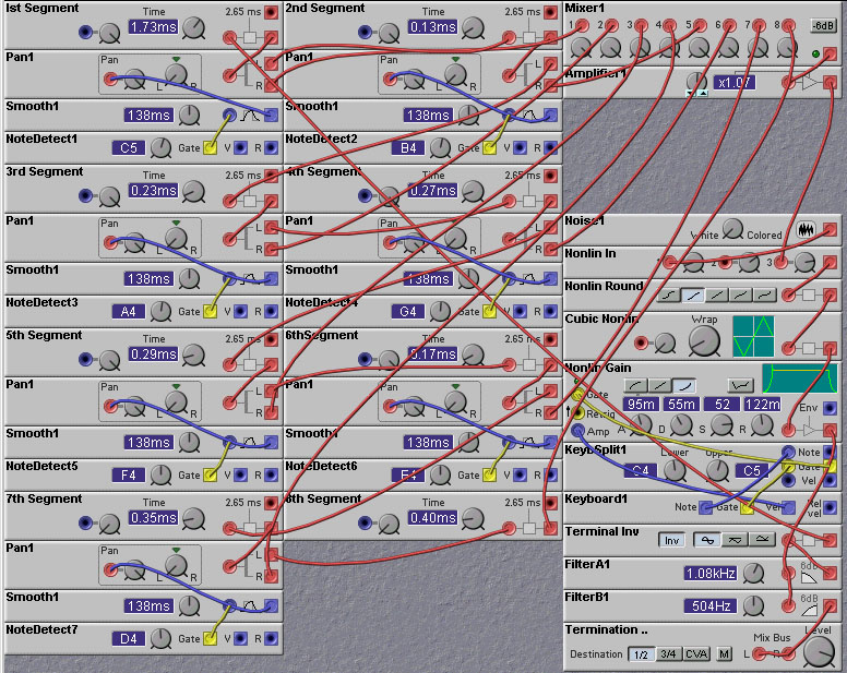
Figure 7.11. A digital waveguide model of a clarinet with toneholes
(J. Clark).
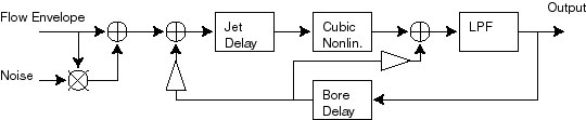
Figure 7.12. Cook's physical model of a slide-flute.
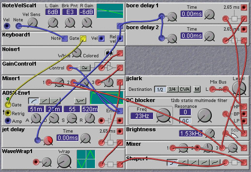
Figure 7.13. Nord Modular implementation of Cook's slide flute model
(J. Clark).
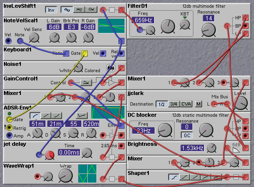
Figure 7.14. A slide flute model using all-pass delay lines (J. Clark).
7.8 Related Links
This chapter has just given the briefest of overviews of physical modelling
of instruments. There are many, many, more details and issues to be
considered, and many other instruments to be analyzed (such as brass instruments
and percussion). If you are interested in implementing more complex
physical models there is a wealth of literature on the topic.
A good introduction to physical modeling can be found at
harmony-central.com/Synth/Articles/Physical_Modeling.
For a thorough analysis of the subject of interpolation in delay lines, see the paper "Discrete-Time Modeling of Acoustic Tubes Using Fractional Delay Lines", by Vesa Välimäki, available at www.acoustics.hut.fi/~vpv/publications/vesa_phd.html.
Rob Hordijk has a good overview of the Nord Modular delay lines at www.clavia.se/nordmodular/Modularzone/DelayModule.html
Chet Singer (creator of many wonderful physical model patches for the Nord Modular) provides the following links:
1.
http://www-ccrma.stanford.edu/software/clm/compmus/clm-tutorials/pm.html
This has examples of
the Karplus-Strong algorithm and a flute. The flute is difficult to tune
on the NM, because there are two different waveguides in it, and they must
be precisely tuned one octave apart.
2.
http://ccrma-www.stanford.edu/~jos/
This is Julius Smith's home
page. He didn't invent physical modeling, but he's probably advanced
it as far, or further, than anyone else.
3.
http://www-ccrma.stanford.edu/~jos/waveguide/waveguide.html
This is a particularly good document within Julius Smith's home page. It's huge.
Some of it gets kind of deep, but it also includes block diagrams of
clarinets and violins.
4.
http://www-ccrma.stanford.edu/software/stk/
If you're familiar with computer programming, this is Perry Cook's
Synthesis ToolKit software package. It contains some examples of physical
models written in C++.
5.
http://windsynth.org/iwsa_labs/patch_programming/prog_techniques/VL1_Guide/
This is a VL programming guide. There's some interesting information in
here, especially after reading some of Julius Smith's stuff, and some of the
Yamaha patents.
6.
http://www.delphion.com
This is a patent search site.
Some relevant US patents are:
5,117,729: basic woodwind, brass, and a synthetic wind instrument model.
5,157,216: using pulsed noise for simulating bow scraping.
5,272,275: really complicated brass model.
5,286,914: multiple-model instrument. I think it's the VL1.
5,438,156: modeling a conical tube.
5,508,473: simulating period-synchronous noise in a wind instrument.
5,748,513: using coupled waveguides to create inharmonic sounds.
6,175,073: an improved bowed model.
These are all either Yamaha or Stanford patents. A list of the Stanford patents can be found at http://www.sondiusxg.com/patent.html.
7. M. E. McIntyre, R. T. Schumacher, and J. Woodhouse. "On the Oscillations of
Musical Instruments". J. Acoust. Soc. Amer.,
Vol. 74, No. 5, pp. 1325-1345, 1983.
introduced the driver-and-waveguide idea. It describes a clarinet, a
bowed string, and a flute.
8.
http://www.sospubs.co.uk/sos/1997_articles/jul97/ronberry.html
This describes some work done by Ron Berry on implementing
physical modeling on his modular analog synth.
