Figure 6.1. A basic patch that can be used as a template for additive designs (J. Clark).
Additive synthesis is a technique which builds sounds from the bottom up, by incrementally adding simple waveforms together to achieve the desired resultss. Additive synthesis can be used to very accurately model almost any musical instrument, given enough computational resources. Computational resources are limited on the Nord Modular, however, implying that perfect emulations of instruments will not be achievable. But, very good results can be obtained in some cases!
Besides the high demand on computational resources, additive synthesis has some implementational quirks which can affect the quality of the synthesized sound. One of these arises from the fact that a large number of sound sources are being added together. Since each of these sound sources has some noise, adding them together will neccessarily increase the noise level. Compare this to the situation in subtractive synthesis where the output noise can be less than the noise level of the input waveform, due to the filtering. Thus, instruments created using additive synthesis can be noisy. Another factor to consider is the relative fragility of the harmonic structure of the additive sound. If the user has some control over some aspect of the additive process, say in the amplitude or frequency of some overtone, the complex harmonic structure that provides a certain type of sound can be destroyed, leading to a thin sound. In fact, one of the main criticisms of additive synthesizers is that they produce rather thin sounds. This is not an problem with additive synthesis per se - additive synthesis does have the capability to make rich powerful sounds. The problem is that the characteristics of the overtones must be carefully and precisely set in order to achieve such sounds. It may be difficult to do this just by manually adjusting the sound parameters. Resynthesis based on mathematical analysis of the target sound is usually required to obtain good results. Another problem with additive synthesis is that transient sounds are very difficult to synthesize. This is because transients require a large number of rapidly varying overtones to obtain accurate reconstructions. The phase relationships between the various oscillators must also be carefully controlled to get a sharp attack. Even though the harmonic structure of a sound does not depend on the relative phases of the individual oscillators (except in rare cases of complete cancellation), temporal events such as rapid attacks or decays are very much dependent on the oscillators phases. Noisy instruments, such as drums, flutes, and cymbals, are also hard to synthesize, again due to the large number of overtones required. One can overcome this difficulty somewhat by modulating the overtone frequencies and amplitudes with noise signals. This has the effect of spreading the sinewave frequency, which is itself just an impulse in the frequency domain, to a broader range of frequencies. In general, however, additive synthesis is at its best when synthesizing sounds that are quasi-periodic.
The basic additive synthesis patch is shown below.
Re-synthesis is not a simple process, even for computers. It is often difficult to detect spectral peaks, as the peaks may widen and merge with others, or be weak. Tracking peaks from one time segment to the next is also a difficult problem, as peaks may be created, disappear, or merge with other peaks. Nonetheless, quite good results can be obtained. This is not something that the Nord Modular is capable of doing itself, at least not with sufficient accuracy. One could write a computer program that would take in a wave file containing an instrument sample and spit out a Nord Modular patch (similar to that of figure 1) which would give an additive synthesis approximation to the sound. If you, or someone close to you, ever writes such a program, let me know!
If you are the patient type, you could try to do re-synthesis by hand, from a table or chart of partial frequencies and amplitudes. Since partial amplitudes in such charts are usually expressed in decibels (dB), it is neccessary to know the attenuation of the mixer and/or sine-bank level controls in dB. Ico Doornekamp has tabulated a list of gain values for the Nord Modular mixer level control in dB. Apparently (although I have not confirmed this) the same conversion factor can be used for the level control in the sinebank oscillator. The values are as follows:
| 127 1.00000 0.000 | 126 0.97852 -0.094 | 125 0.94617 -0.240 | 124 0.91984 -0.363 | 123 0.89383 -0.487 | 122 0.86836 -0.613 | 121 0.84320 -0.741 | 120 0.81852 -0.870 |
| 119 0.79414 -1.001 | 118 0.77023 -1.134 | 117 0.74680 -1.268 | 116 0.72370 -1.404 | 115 0.70109 -1.542 | 114 0.67883 -1.682 | 113 0.65703 -1.824 | 112 0.63570 -1.967 |
| 111 0.61480 -2.113 | 110 0.59422 -2.261 | 109 0.57406 -2.410 | 108 0.55445 -2.561 | 107 0.53523 -2.715 | 106 0.51641 -2.870 | 105 0.49805 -3.027 | 104 0.48008 -3.187 |
| 103 0.46250 -3.349 | 102 0.44539 -3.513 | 101 0.42867 -3.679 | 100 0.41237 -3.847 | 99 0.39648 -4.018 | 98 0.38102 -4.191 | 97 0.36602 -4.365 | 96 0.35133 -4.543 |
| 95 0.33711 -4.722 | 94 0.32328 -4.904 | 93 0.30984 -5.089 | 92 0.29680 -5.275 | 91 0.28431 -5.462 | 90 0.27183 -5.657 | 89 0.25787 -5.886 | 88 0.24391 -6.128 |
| 87 0.23461 -6.297 | 86 0.22530 -6.472 | 85 0.21600 -6.655 | 84 0.20425 -6.898 | 83 0.19249 -7.156 | 82 0.18466 -7.336 | 81 0.17682 -7.525 | 80 0.16898 -7.722 |
| 79 0.15923 -7.980 | 78 0.14948 -8.254 | 77 0.14298 -8.447 | 76 0.13648 -8.649 | 75 0.12998 -8.861 | 74 0.12204 -9.135 | 73 0.11409 -9.427 | 72 0.10880 -9.634 |
| 71 0.10350 -9.851 | 70 0.09820 -10.079 | 69 0.09186 -10.369 | 68 0.08551 -10.680 | 67 0.08128 -10.900 | 66 0.07705 -11.132 | 65 0.07282 -11.377 | 64 0.06784 -11.685 |
| 63 0.06286 -12.017 | 62 0.05953 -12.252 | 61 0.05621 -12.502 | 60 0.05289 -12.766 | 59 0.04907 -13.092 | 58 0.04525 -13.444 | 57 0.04270 -13.696 | 56 0.04015 -13.963 |
| 55 0.03760 -14.248 | 54 0.03517 -14.539 | 53 0.03273 -14.850 | 52 0.03030 -15.186 | 51 0.02820 -15.498 | 50 0.02609 -15.835 | 49 0.02399 -16.200 | 48 0.02189 -16.598 |
| 47 0.02049 -16.885 | 46 0.01908 -17.193 | 45 0.01768 -17.524 | 44 0.01618 -17.909 | 43 0.01468 -18.332 | 42 0.01368 -18.639 | 41 0.01268 -18.969 | 40 0.01168 -19.326 |
| 39 0.01063 -19.734 | 38 0.00958 -20.185 | 37 0.00888 -20.514 | 36 0.00818 -20.870 | 35 0.00748 -21.258 | 34 0.00678 -21.689 | 33 0.00607 -22.168 | 32 0.00560 -22.519 |
| 31 0.00513 -22.900 | 30 0.00466 -23.320 | 29 0.00419 -23.774 | 28 0.00373 -24.281 | 27 0.00342 -24.657 | 26 0.00311 -25.067 | 25 0.00280 -25.521 | 24 0.00251 -25.999 |
| 23 0.00222 -26.539 | 22 0.00202 -26.939 | 21 0.00183 -27.380 | 20 0.00163 -27.871 | 19 0.00145 -28.377 | 18 0.00128 -28.945 | 17 0.00115 -29.375 | 16 0.00104 -29.847 |
| 15 0.00092 -30.383 | 14 0.00081 -30.919 | 13 0.00070 -31.520 | 12 0.00063 -31.987 | 11 0.00056 -32.499 | 10 0.00049 -33.079 | 9 0.00044 -33.590 | 8 0.00038 -34.170 |
| 7 0.00034 -34.677 | 6 0.00030 -35.274 | 5 0.00025 -35.940 | 4 0.00022 -36.478 | 3 0.00019 -37.128 | 2 0.00017 -37.768 | 1 0.00015 -38.285 | 0 0.00000 -infinity |
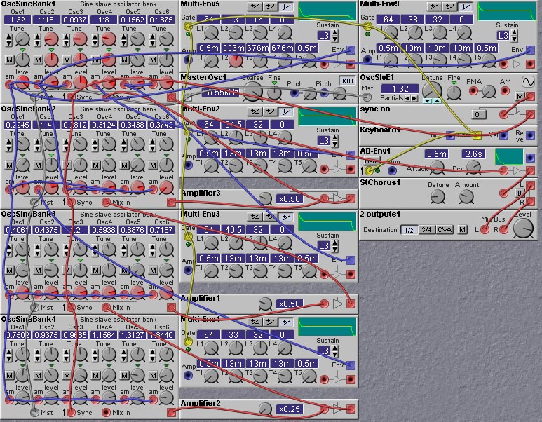
Figure 2 shows an additive synthesis patch that divides 24 partials into 5 groups, each with its own amplitude envelope. A manual re-synthesis approach was taken for the design of this patch. A piano sample was examined using the spectral analysis capabilites of Cool-Edit. Spectra were obtained at 50 millisecond intervals over the length of the sample (to give 20 spectra for a one second long sample). First, a spectrum from near the middle of the sample was examined to determine the location of the strongest spectral peaks. The relative amplitudes (in dB) of these peaks were measured. These amplitudes were used to set the levels of the sine-bank oscillators, using the conversion factor given in table 6.1. Then, the peaks were tracked (manually!) in the other time window spectra by a nearest-neighbor heuristic (the peaks don't shift very much in this sample) and their amplitudes roughly plotted. The partial groups were assigned from the amplitude plots by grouping together spectral peaks whose amplitude curves looked qualitatively similar. Multi-stage envelope modules were used to implement amplitude curves that more-or-less matched the general shape of the partial amplitude plots. The resulting sound is something like a piano, at least more like a piano than a saxophone. The sound is rather organ-like, a common result of additive synthesis.
A solution to the problem of adding expressiveness to additive synthesis is morphing, where the performer controls a morph, or smooth transition, between two different sets of additive synthesis parameters. One could also use an approach similar to wave-terrain synthesis, in which the performer specifies a one-dimensional trajectory or curve in the high-dimensional space of additive synthesis parameters. Different points in this space correspond to different sounds, and in this way the performer can move from one sound to the next.
Morphing can be accomplished in many ways. Two of the most common are cross-fading of two different waveforms, and varying, in a concerted manner, a number of parameters between two different settings. In the Nord Modular the cross-fade module can be used to implement the first type, while the Morph controller groups can be used to implement the second type. It is greatly preferable to use the Morph controller group than cross-fading, as cross-fading requires duplication of most of the patch. Besides using the Nord Modular morph groups, morphing of voltage-controllable parameters can be implemented using cross-fading of the parameter values between two different levels. This approach is more tedious to implement than the morph groups but is very flexible, and can control a large number of parameters, whereas the morph groups are limited to controller a maximum of 25 parameters in the Nord Modular.
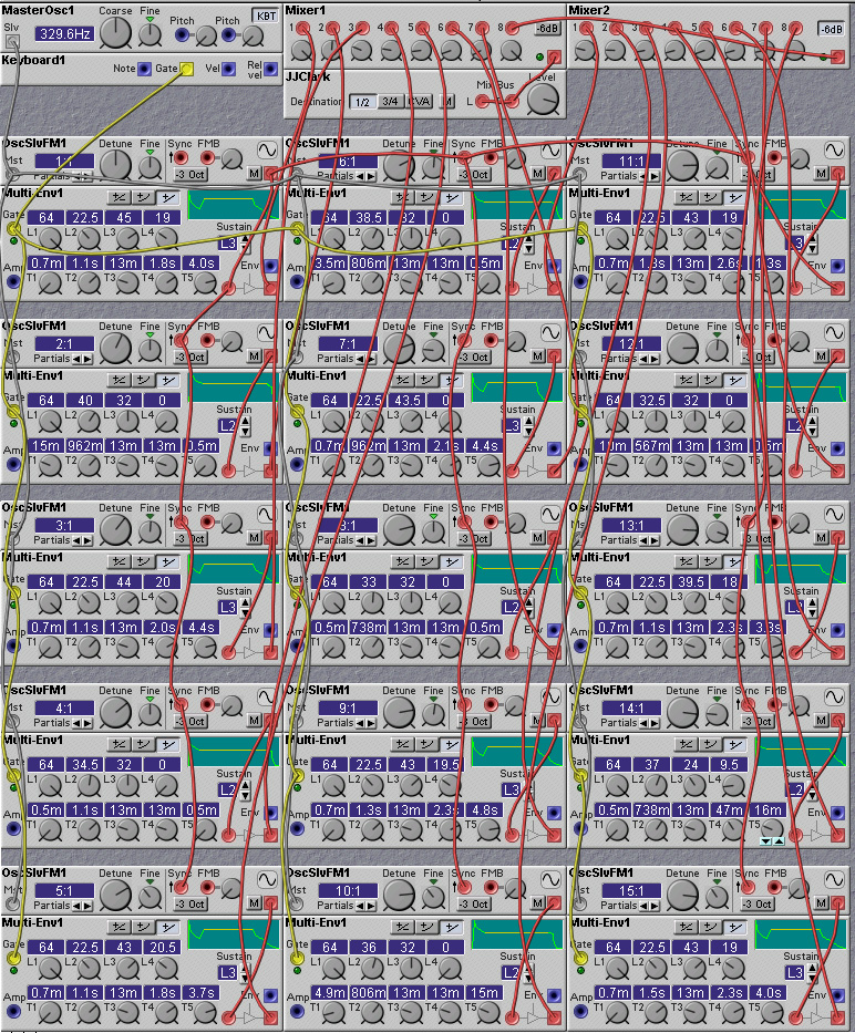
The patch shown in figure 6.2 is an example of such a morphing approach. The morph group is assigned to knob 1 in this patch, but could also be assigned to a MIDI controller such as key velocity or aftertouch. The sound morphs from the (re-synthesized) piano sound to a rather clangourous sound. Note the switch (controlled by knob 2) that enables syncing of the oscillators. When the morph knob is fully clockwise (to play the piano sound), the sync switch has little effect. This is because most of the partials are harmonic. When the morph knob is fully clockwise, so that the clangorous sound is being played, the sync switch has a significant effect.
In this patch, an impulsive noise burst and a short pulse-wave transient are mixed with a simple 5-voice additive synthesis sound. The fifth partial of the additive part is implemented with a pulse generator rather than with a sine-wave. This is a useful trick when you have a limited number of partials to work with - let the highest partial be a non-sinusoidal wave, with lots of harmonics. This non-sinusoidal partial then fills in the higher harmonics. Otherwise, the sound would be dull and lacking in sparkle. A couple of LFOs are added to give some extra motion to the sound.
The slave sinewave oscillator is good for additive synthesis for a
number of reasons:
- It produces a single sinusoidal harmonic.
- It is the single oscillator that uses the least DSP cycles (3%), and
uses just a bit more DSP resources than 1/6 of the sine-bank.
- It has an FM input, which can be used to provide dynamic variation
of the pitch of the partial.
- It has an AM input, which can be used to control the amplitude of
the partial.
The slave FM sinewave oscillator is also very good for additive synthesis. It is slightly more expensive in terms of DSP usage than the non-FM slave sinewave oscillator (3.2% vs. 3.0%) but has one important advantage, that is, it has oscillator sync. This can be used to ensure that all harmonic partials will have a fixed relative phase. Be careful in using oscillator sync on non-harmonic partials, as this will introduce extra harmonics which will be hard to control (of course, these extra harmonics might just give you that sound you are looking for!). The FM sine slave oscillator also has an FM input, which can be used to provide dynamic variation of the pitch of the partial. Use this carefully if you are also using oscillator sync, as the FM then will not cause a change in pitch, but will create extra harmonics.
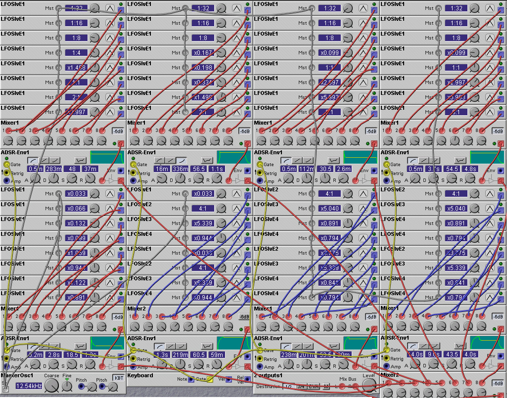
The number of oscillators that we can use in a Nord Modular additive synthesis patch is limited by the available DSP resources. But what if your grand scheme for the greatest patch ever requires more oscillators than this? Well, one way to get a larger number of oscillators is to go cheap and dirty and use LFO modules as the partial generators. An example is shown in the patch below, which uses 64 slave LFOs. You could probably squeeze in more oscillators, but I think you get the point. Triangle oscillators are used as they use the least DSP cycles of any of the LFO slave oscillators. Triangle waves have some low-amplitude higher harmonics, which limits the types of sounds that can be achieved. This slight drawback is insignificant in face of the other drawbacks of using the LFO slave oscillators - the aliasing that is present at higher frequencies, and the limited control one has over the frequency of the harmonics. This patch seems best for generating noisy clangourous sounds! One might question the use of audio mixers in this patch. Wouldn't it be cheaper to use control mixers? Yes, it would, but it would not make any difference to the overall number of oscillators or polyphony that we can achieve, since this is set by the zero-page usage rather than by DSP cycles. And using 8-input audio mixers is much more convenient and simpler to wire up than the 2-input control mixers that are available. You need 7 of these control mixers to construct an 8-input mixer, and the amount of wiring is considerable. Note that group synthesis is used in this patch - the oscillators are partitioned into groups of eight, and each group is amplitude modulated by a single envelope generator.