


Next: Example 2: Finite dimensional
Up: Example 1: Stabilization of
Previous: Step 1: Construction of
Contents
The derivation of the Wei-Norman equation is carried out in two steps. The product term in the right-hand side of (10) is first computed by invoking the LTP function wner, in which the basis elements  need to be replaced by
  ,
,
 . Next, the coefficients corresponding to the basis elements , on both sides of equation (10)-(3) are equated using the LTP function
 wnde.
More precisely, the LTP function wner ought to be invoked with the following parameters:
rhwne:=wner( ,
, ,
, ,
,  , lbdt), where
  is the dimension of the basis ,
  is the degree of nilpotency, and lbdt is the list of linear dependencies . The resulting expression is:
The function wnde(rhwne,,,lbdt) is applied to the above result returning the matrix 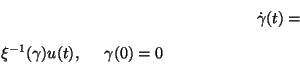 (see equation (12)) and the set of equations:
The inversion of results in the following Wei-Norman equation:
with  ,
,
 .
A feasible control
.
A feasible control  satisfying the inclusion (28) is found as follows. First, (29) is integrated symbolically over
 ![$[0,T]$](img145.png) and solved with respect to the extended controls
and solved with respect to the extended controls  ,
,  evaluated at
  to yield a symbolic expression for the reachable set
 , now given as a set of admissible coordinate values
 for the original system. Next, a control is found by solving (28) using standard nonlinear programming techniques; see [26] for details of this calculation. Stabilization is achieved by repetitive solution of (28) as shown by simulation results in Figure 1 which correspond to an initial condition
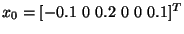
![$x_0=[-0.1\ 0\ 0.2\ 0\ 0\ 0.1]^T$](img406.png) . These results were obtained using a quadratic Lyapunov function
. These results were obtained using a quadratic Lyapunov function
 and piece-wise constant controls consisting of at most five switching times in any interval of length
 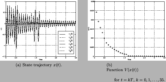 .
.
Figure 1:
Results for the stabilization of the rigid body.
 |
Next: Example 2: Finite dimensional
Up: Example 1: Stabilization of
Previous: Step 1: Construction of
Contents
Miguel Attilio Torres-Torriti
2004-05-31
![\begin{eqnarray*}
rhwne&{:=}&
\dot{\gamma}_0 f_0 + \dot{\gamma}_1 f_1 + \dot{...
...mma}_5 \gamma_0 a + \dot{\gamma}_6)
[[f_0, f_1], [f_0, f_2]]
\end{eqnarray*}](img397.png)
![$\displaystyle \left [\begin{array}{c}\dot{\gamma}_0\\ \dot{\gamma}_1\\ \dot{\...
...ma}_3\\ \dot{\gamma}_4\\ \dot{\gamma}_5\\ \dot{\gamma}_6
\end{array}\right ]$](img399.png)