(1)
The Viterbi Algorithm
I
n this section we will describe the Viterbi algorithm in more detail. The Viterbi algorithm provides an efficient way of finding the most likely state sequence in the maximum a posteriori probability sense of a process assumed to be a finite-state discrete-time Markov process. Such processes can be subsumed under the general statistical framework of compound decision theory. We proceed to explain this theory in the context of Text Recognition as defined in [3], since this is the application that we will focus on later on.Compound decision theory
S
uppose we have a text of n characteres. Each character yields a feature vector zi, i=1,2,...,n. Let p(Z|C) denote the probability density function of the vector sequence Z=z1,z2,...,zn conditioned on the sequence of identities C=c1,c2,...,cn, where zk is the feature vector for the k-th character, and where ck takes on M values (number of letters in the alphabet) for k=1,2,...,n. Also, let P(C) be the a priori probability of the sequence of values C. In other words P(C) is the a priori probability distribution of all sequences of n characters. The probability of correctly classifying the text is maximized by choosing that sequence of characters that has a maximum posterior probability or the so called: maximum a posteri (MAP) probability, given by P(C|Z).F
rom Bayes' rule we obtain|
|
(1) |
S
ince p(Z) is independent of the sequence C (it is just a scale factor) we need only maximize the discriminant function|
|
(2) |
T
he amount of storage required for these probabilities is huge in practice, for that reason, assumptions are made in order to reduce the problem down to manageable size. These assumptions are:![]() The size of the
sequence of observations is not very large. Let n be the size of a word. Then P(C) is the frequency of occurrence of words.
The size of the
sequence of observations is not very large. Let n be the size of a word. Then P(C) is the frequency of occurrence of words.
![]() Conditional independence among the features vectors. The shape of a character, which generates a given feature vector, is independent of the shapes of neighbouring characters and is, therefore, dependent only on the character in question.
Conditional independence among the features vectors. The shape of a character, which generates a given feature vector, is independent of the shapes of neighbouring characters and is, therefore, dependent only on the character in question.
U
nder these assumptions, and taking logarithms, Eq. 2 reduces to|
|
(3) |
F
or the case of the Viterbi algorithm, if we assume that the process is first-order Markov, then Eq. 3 reduces to:|
|
(4) |
T
he MAP sequence estimation problem previously stated can also be viewed as the problem of finding the shortest route [1] through a certain graph. By thinking in this similarity one can see the natural recursivity of the Viterbi algorithm.T
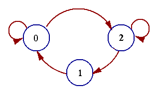
o illustrate how the Viterbi algorithm obtains this shortest path, we need to represent the Markov process in an easy way. A state diagram, like one shown in Fig. 2, is often used. In this state diagram, the nodes (circles) represent states, arrows represent transitions, and over the course of time the process traces some path from state to state through the state diagram.
Fig. 2 State diagram of a three-state process.
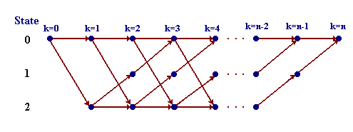
A more redundant description of the same process is shown in Fig. 3, this description is called trellis. In a trellis, each node corresponds to a distinct state at a given time, and each arrow represents a transition to some new state at the next instant of time. The trellis begins and ends at the known states c0 and cn. Its most important property is that to every possible state sequence C there corresponds a unique path through the trellis, and vice versa.

Fig. 3 Trellis for the three-state process of Fig. 1.
Now, suppose we assign to every path a length
proportional to -log [p(Z|C)+P(C)]. Since log() is a monotonic function and there is a one-to-one correspondence between paths and sequences, we only need to find the path whose -log [p(Z|C)+P(C)] is minimum, this will give us the state sequence for which p(Z|C) P(C) is maximum, in other words, the state sequence with the maximum a posteriori (MAP) probability, which take us back to the original problem we want to solve. The total length of the path corresponding to some state sequence C is
where
l(tk ) is the associated length to each transition tk from ck to ck+1. The shortest such path segment is called the survivor corresponding to the node ck, and is denoted S(ck). For any time k>0 , there are M survivors in all, one for each ck. The observation is this: the shortest complete path S must begin with one of these survivors. Thus for any time k we need to remember only the M survivors S(ck) and their correspondent lengths. To get to time k+1, we need only extend all time-k survivors by one time unit, compute the lengths of the extended path segments, and for each node ck+1 as the corresponding time-(k+1) survivor. Recursion proceeds indefinitely without the number of survivors ever exceeding M. This algorithm is a simple version of forward dynamic programming.W
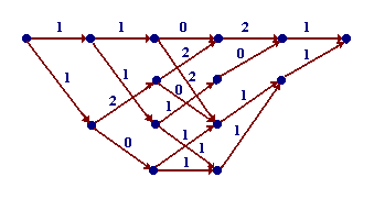
e illustrate this with an example taken from [1] that involves a four-state trellis covering five time units. The complete trellis with each branch labeled with a length is shown in Fig. 4.
Fig. 4 Trellis labeled with branch leghts; M=4, n=5
T
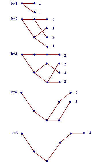
he 5 recursive steps by which the algorithm determines the shortest path from the initial to the final node are shown in Fig. 5. At each step only the 4 (or fewer) survivors are shown, along with their lengths.
Fig. 5 Recursive determination of the shortest path via the Viterbi algorithm.
T
he Viterbi algorithm seen as finding the shortest route through a graph is:|
Input: |
|
|
|
|
|
Z=z1,z2,...,zn |
|
the input observed sequence |
|
Initialization : |
|
|
|
|
|
k=1 |
|
time index |
|
|
S (c1)=c1 |
|
|
|
|
L (c1)=0 |
|
this is a variable that accumulate the lengths, the initial length is 0 |
|
Recursion: |
|
|
|
|
For all transitions tk=(ck,ck+1) |
|
|
|
compute: L(ck,ck+1) = L(ck) + l [tk = (ck,ck+1)] among all ck. |
|
|
Find L(ck+1) = min L(ck,ck+1) |
|
|
For each ck+1 |
|
|
store L(ck+1) and the corresponding survivor S(ck+1). |
|
|
|
k=k+1 |
|
|
|
Repeat until k=n |
|
W
ith finite state sequences C the algorithm terminates at time n with the shortest complete path stored as the survivor S(cK).T
he complexity of the algorithm is easily estimated:![]() Memory: the algorithm requires M storage locations, one for each state, where each location must be capable of storing a length L(m) and a truncated survivor listing S(m) of the symbols.
Memory: the algorithm requires M storage locations, one for each state, where each location must be capable of storing a length L(m) and a truncated survivor listing S(m) of the symbols.
![]() Computation: in each unit of time the algorithm must make M2 additions at most, one for each existing transition, and M comparisons among the M2 results.
Computation: in each unit of time the algorithm must make M2 additions at most, one for each existing transition, and M comparisons among the M2 results.
T
hus, the amount of storage is proportional to the number of states, and the amount of computation to the number of transitions.