Consider a Markov chain \(\{X_t, t= 1, 2, \dots \}\) with state space \(\mathcal X = \{0, 1\}\) and matrix of transition probabilies shown below.
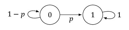
The state \(0\) denotes a safe state while the state \(1\) denotes a faulty state. Assume that \(\PR(X_1 = 0) = q_0\).
A decision makers observes the state with noise as follows \[ Y_t = h(X_t, N_t), \quad t= 1, 2, \dots\] where \(\{N_t\} _ {t=1}^{T}\) is the observation noise process and \(h\) is a known function. It is assumed that all primitive random variables are mututally independent.
Let \(\theta\) denote the (random) time at which the Markov chain jumps from state \(0\) to state \(1\) (with \(\theta = 0\) is the Markov chain starts in state \(1\)).
At each time step, the decision maker has two alternatives: stop and declare that a fault has occured (denoted by \(u_t = 1\)) or take another measurement (denoted by \(u_t = 0\)). The system runs for a finite horizon \(T\). Let \(\tau\) denote the (random) time the decision maker declares that the jump has occured (if the decision maker does not declare to stop, then \(\tau\) is assumed to be \(T+1\)).
The objective is to determine the strategy of the decision maker that minimizes the exptected cost \[ \EXP^{\bf g} [ \IND(X _ \tau = 0) \IND (\tau < T + 1) + k \sum_{t=0}^{\tau - 1} \IND(X_t = 1) ]\] where \(k\) is a poistive constant, and \(\IND(\cdot)\) is an indicator function.
Show that the above model is a POMDP. Identify an information state, and write the dynamic programming decomposition.
Show that an optimal strategy \(g\) is of the following form:
- If \(\PR(\theta > t | Y _ {1:t} ) > \ell_t\), continue;
- If \(\PR(\theta > t | Y _ {1:t} ) \le\ell_t\), stop and declare that the fault as occured.
Specify the equations that determine the thresholds \(\ell_t\), \(t=1,\dots,T\).
A missing aircraft is assumed to have crashed in the ocean. The search area is divided into \(n\) cells. For each cell \(i\), denote by:
- \(c_i\): the cost to search in cell \(i\)
- \(p_i\): the prior probability that the aircraft is in cell \(i\)
- \(\alpha_i\): Conditioned on the event that the aircraft is in cell \(i\), the probability that it is detected when cell \(i\) is searched.
Thus, examining cell \(i\) costs \(c_i\) unit per time and reveals the object (if it is there) with probability \(\alpha_i\).
The aircraft is sequentially serach one cell at a time. The search terminates if the aircraft is found or if we have searched \(T\) times, whichever is earlier. The objective is to identify an optimal search strategy for finding the aircraft at minimum cost.
Let \(q_i(t)\) denote the posterior probability that the aircraft is in cell \(i\) at time \(t\) given the history of all search locations and the event that the aircraft has not been found so far. Suppose we search location \(k\) at time \(t\) but do not find the aircraft. Write an expression for \(q_i(t+1)\) in terms of \(q_i(t)\) (consider \(i = k\) and \(i \neq k\)).
Suppose the aircraft is searched at location \(k\) at time \(t\), and if not found, then it is searched in location \(\ell\) at time \(t+1\), where \(k \neq \ell\). Write an expression for the expected cost of search for time \(t\) and \(t+1\) in terms of \(q_k(t)\) and \(q_\ell(t)\).
Using an interchange argument to find an optimal search order.
In the static team problem discussed in class, we assumed that \((X, Y^1, \dots, Y^n)\) were zero-mean Gaussian random variables. Now suppose that they are not zero mean. In particular, let \(\EXP[X] = \bar x\) and \(\EXP[Y^i] = \bar y^i\). Show that a control law of the form \[ U^i = K^i(Y^i - \bar y^i) + H^i \bar x\] is optimal. Find equations to compute \(K^i\) and \(H^i\).