Consider the graph shown below. At each node (except the nodes at stage 3), the decision maker has three actions: \(U\), \(M\), and \(L\). The cost associated with each action is shown on the edge. Suppose we are interested in minimizing the cost of choosing a path from \(x_0\) to \(x_T\).
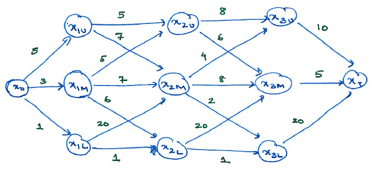
Weighted graph
- Find the value functions at time \(t=3,2,1\).
- Identify the optimal strategy.
- Identify the shortest path from \(x_0\) to \(x_T\).
A hunter is interested in optimal scheduling of hunting during an expedition that may last up to \(T\) days. The hunter has two options on each day: he may go out to hunt or he may decide to stop the expedition and go back home.
- Going out to hunt costs \(c\) units per day with the possibility of capturing one animal. The probability of capture depends on the population \(n\): probability of a capture is \(p(n)\); probability of no capture is \(1 - p(n)\). In case of a capture, the hunter gets a reward of one unit; otherwise, he gets no reward.
- If he decides to stop the hunting expedition, the hunter does not get any opportunity to hunt in the future, and as such receives no reward in the future. There is no cost associated with taking this action.
- The hunter must return back at the end of \(T\) days.
Assume the following:
- The hunter knows the initial population \(N\).
- The time scale is such that the population does not change due to natural causes (birth or death).
- The probability that the hunter makes more than one capture a day is negligible.
- The function \(p(n)\) is monotonically increasing in \(n\).
For the above system:
Write a dynamical model with the state as the current population. Argue that the above system is a MDP and write the dynamic program for this system.
Note: You can write the dynamic program in two ways: either to maximize reward or to minimize cost. You may use either of these alternatives.
Let \(λ\) be the smallest integer such that \(p(λ) > c\). Show that it is optimal to stop hunting when the current population falls below \(λ\).
Hint: The above result is equivalent to saying that the value function is zero if and only if the current population is less than \(λ\).
Consider the example of optimal power-delay trade-off in wireless communication described in the class notes. For that model, prove the following:
\(\forall t\): \(V_t(x,s)\) is increasing in \(x\) for all \(s\); and decreasing in \(s\) for all \(x\).
\(\forall t\): \(V_t(x,s)\) is convex in \(x\) for all \(s\).
Let \(\mathbf g^ * = (g^ * _ 1, \dots, g^ * _ T)\) be an optimal strategy. Then, \(\forall t\): \(g^ * _ t(x,s)\) is increasing in \(x\) for all \(s\).
In order to prove the convexity of the value function, you might find the following characterization useful. Let \(\mathcal X\) be a discrete space. Then, the following are equivalent:
- \(f\) is convex.
- \(f(x+1) - f(x)\) is increasing in \(x\).
- \(f(x) + f(y) \ge f(\left\lfloor \frac{x+y}{2} \right\rfloor) + f(\left\lceil \frac{x+y}{2} \right\rceil)\) for all \(x,y \in \mathcal X\).