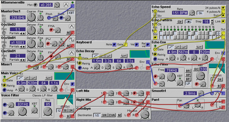
Figure 11.1. Echo patch using a retriggered envelope (M. Sommerville).
So then, what is a poor synthesist to do?? We need our reverbs! There are a number of options. The best option is to use an external effects unit to provide reverb and echo. You can use the analog outputs of the Nord Modular to route signals to the external effects, and can use the analog inputs of the NM to feed the processed signals back in (especially useful with echo effects).
But is it possible to do something with the Nord Modular, to produce reverb or echo effects? Well, yes, there are some things that can be done. I will discuss these in the following sections.
The Nord Modular is often used to generate sounds internally, rather than to process external sounds. In this case we can modify the sound generation process to directly produce the required echoes and reverberations. To make this clear, consider the following simple example - suppose we want to generate a simple single oscillator sound, but with an adjustable echo effect. Instead of constructing a patch using a single VCA and envelope generator, with a long delay line, we could use multiple envelope generators (or a single multi-stage envelope) to create the echoes. You could also use a single envelope, but retrigger it repeatedly to produce the echoes. You should decrease the overall amplitude of the sound, perhaps with another envelope, to mimic the decay of the echoes. This technique is used in the following patch (by Martin Sommerville). In this patch, an event sequencer is used to specify when the echoes are generated. This allows an irregular spacing of the echoes, giving an effect similar to reverberation.
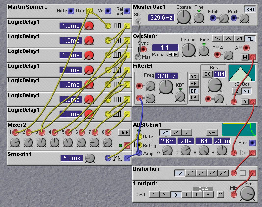
Logic delay modules can also be used in creating synthetic echo and reverb sounds. This is done in the following patch, also developed by Martin Sommerville. In this patch a set of eight logic delay modules are used to create eight echoes of the keyboard gate signal. These are weighted by the attenuator controls of the mixer module to provide a falloff in amplitude, and frequency content, of the echoes with time. The delayed pulses are used to gate the envelope of the sound.
Similar approaches can be used to create synthetic reverb sounds. In a reverb sound one adds echoes of the primary sound. Unlike a standard echo effect, in a reverb effect the echo times become varied (modeling the various pathways the sound takes as it bounces around the walls of the room) and the sound of the individual echoes become duller and duller (modeling the loss of high frequency information each time sound bounces off of a wall). This approach is shown in the next patch.
The next patch, by Rob Hordijk, is slightly more complicated. It creates a single echo, using a delayed envelope, and then passes the echo through a series of modules which diffuses (or spreads out in time) the echo.
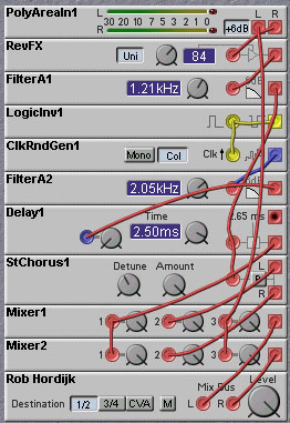
The diffusion is done by a delay line whose delay time is modulated by a randomly varying signal. The LogicInv1 module is wired in a positive feedback arrangement, which produces a high frequency square wave which is used to clock the ClkRndGen1 module. This is a cheap way to generate a clock signal. A chorus is also applied to the echo signal and added to the diffused signal. This thickens up the sound some more. Note that the diffusion is done in the Poly area. This means that the diffusion acts on all of the notes being played at the same time. Thus the reverb effect is on the entire sound being played, rather than on the individual notes.
One can use the audio delay line modules of the Nord Modular to create echoes and reverb. This is the obvious strategy, but one must remember that the delay line module's maximum delay time is quite short, only 2.65 msec. You can only string 10 of them together without exceeding the Nord Modular's memory limits. Thus it would seem that only a 26.5 msec delayline could be made, much too short for a useable echo effect. This short time can be used to make a reverb effect, albeit one which models being in a very small room. An example of this is shown in the following patch, made by Kaspar Thommen.
If we are willing to sacrifice a bit (a lot!) of sound quality there are some tricks that can be played to obtain longer delay times with the Nord Modular. These tricks can then be employed to produce low-fi echo and reverb effects.
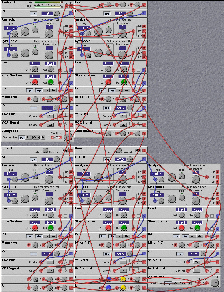
The following patch, designed by Kaspar Thommen, is a clever way to obtain a reverb effect. It basically uses a vocoding process to analyze the input signal, delay the analysis signals with envelope followers, and then resynthesize. This results in delayed versions of the input signal, which can be added to the original input to achieve the reverb effect. The result is not perfect, since the resynthesis of the input is rather crude. But it is still usable for some sounds, like drums. Perhaps if a future update of the Nord Modular software ever provides a vocoder with accessible analysis signals, this patch could be improved.
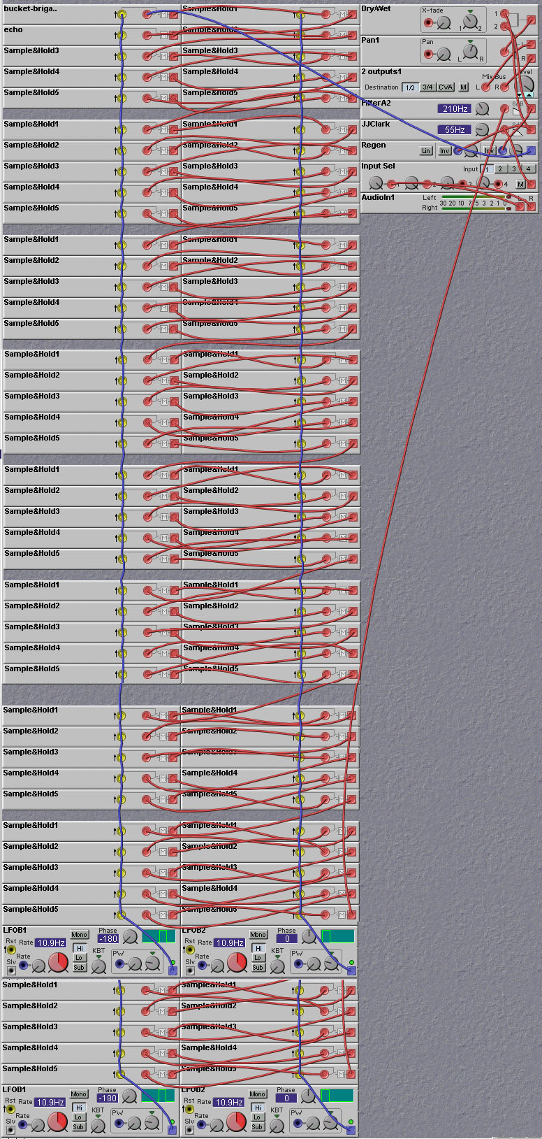
It is possible to make longer delays by trading off sampling rate for delay time. While the Nord Modular delay line modules do not have adjustable sampling rates, we can create our own delay lines using strings of Sample/Hold modules. A string of two S/H modules acts as a delay. Suppose we sample the input to the first S/H and hold it. Then, say T milliseconds later, we sample the output of this S/H with the second S/H. Only then will the input value find its way to the output of the second S/H. Thus there will be a delay of T milliseconds. Of course, the price we pay is that the sampling period of the output is also reduced to T milliseconds. But S/H modules are less resource hungry than the audio delay lines, so we can use more of them. In fact, you can get 98 of them before exceeding the Nord Modular resource limitations. Thus we can string together a whole bunch of these two-S/H delaylines to get one long delay line. This type of delay line structure is known as a Bucket-Brigade delay line (BBD). The name comes from the observation that the action of the sample/hold modules is much like that of the buckets of water used in old fire-fighting brigades, where water was carried in buckets from person to person in a line from the water source to the fire. BBDs are used in many analog chorus and delay effects found on synthesizers and guitar effects boxes. They are usually implemented using Switched-Capacitor or Charge-Coupled-Device (CCD) technology.
The following patch shows a bucket-brigade delay line being used in an echo circuit. It uses 90 S/H modules, giving a delay time of 89 times the sampling period (note: only part of the S/H delay line is shown in the figure below, to save space - download the patch file to see the entire circuit). So, if the sampling period is 5 msec (sample rate of 200 Hz) then the time between echoes is 445 msec. More than enough for a useful echo effect. The main drawback of this patch is that the input signal must be limited in high frequency content to under 1/2 the sampling rate (e.g. 100 Hz in the above example). So the patch is best used for low frequency sounds such as bass drums. To make sure that the input signal's high frequency content is limited, we filter it with a lowpass filter. This is known as anti-aliasing in signal processing terminology, as it prevents the "aliasing" of high frequency components back into lower frequencies when a signal is sampled. Note also the use of control mixers instead of audio mixers for combining audio signals. This reduces the DSP usage and causes very little signal degradation as the signal frequency is low enough to be handled by the lower control sampling rate.
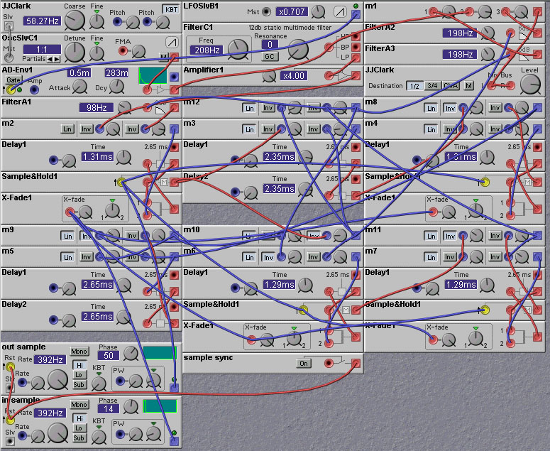
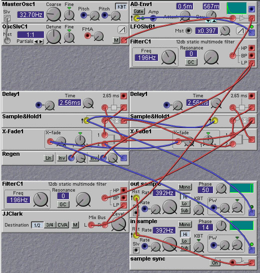
Finally, the audio delay line modules can be coaxed into giving more delay. The trick is to recirculate the signal through the delay line many times. But wouldn't this just overwrite whatever is coming into the delay line? Not if we subsample the input, and interleave it with the delayed signal(s). Interleaving is a technique used in many communication systems (where it is called Time-Division-Multiple-Access, or TDMA) to send many relatively low frequency speech signals over a single high bandwidth communication channel. In our application, we make use of the fact that the audio delay line actually operates at quite a high sampling rate (96KHz). Suppose that we only needed a sampling rate of 9.6KHz. Then, theoretically, we could cram ten of these lower frequency signals into the delay line without them getting in the way of each other. So the idea behind the recirculating delay line is to use one slot for the input signal and the other nine (or however many slots you divide the line into) to hold the recirculating signals. Since, in this example, we have room for nine recirculating signals, the total delay time will be 9 times the nominal delay time of the audio delay line. The following patch does just this - it creates a recirculating delay line, where a crossfader is used to switch the input to the audio delay line module between either the input or the output at appropriate times to do the recirculation. The sample/hold module is used to sample the output at the right time - we only want to sample the output when the data has finished recirculating the desired number of times. The way to ensure this is to sample the output just before reading in the next input sample. The patch is just for demonstration purposes. To alter it for practical use you should remove the test input signal generation modules (the VCO, envelope etc) and replace it with an audio input module. Also add in a crossfader between the input signal and the output of the echo unit to provide a wet/dry mix control.
This patch uses fewer resources than the bucket-brigade echo patch,
but it suffers from the same drawbacks, namely the limited frequency
response. It is also very difficult to adjust the echo time. This is
because the delay time of the recirculating delay line depends
critically on the sampling rate relative to the delay time of the
individual audio delay line modules. For most ratios proper
interleaving is not possible, and the recirculating signals interfere
and overwrite each other. So careful adjustment of the sampling rate
and of the delay line module delay time is needed for proper
operation. The following table lists the total delay values of a
single recirculating delay stage (there are two in the patch shown
above) attained for various delayline delay times, with a sample rate
of 392Hz:
| Delayline Delay Times (msec) | Total Delay (msec) |
| 1.31 | 23 |
| 1.29 | 39 |
| 2.65 | 54 |
| 2.60 | 88 |
| 2.58 | 129 |
| 2.56 | 245 |
You can see that the total delay time does not vary linearly with the delay module time, as you might expect. This is because the number of recirculations is equal to:
| 0000 (initially delay line is all zero) |
| 1000 <- 1 (first input) |
| 0100 (recirculate) |
| 0010 (recirculate) |
| 0001 (recirculate) |
| 1000 (recirculate) |
| 0100 -> 0 (sample output and recirculate) |
| 2010 <- 2 (second input) |
| 0201 (recirculate) |
| 1020 (recirculate) |
| 0102 (recirculate) |
| 2010 (recirculate) |
| 0201 -> 1 (first input makes it to the output after 11 time steps) |
| 3020 <- 3 (third input) |
| 0302 (recirculate) |
| etc... |
The output is sampled one time unit before the input is sampled (and fed into the delay line). The total delay for this example is seen to be 11 time units. This is equal to (T_D*T_R/GCD(T_D,T_R))-1 = (4*6/GCD(4,6))-1 = (4*6/2)-1 = 11.
For a more detailed example, suppose the recirculation clock period T_R is 1/392Hz = 2.55 msec, and the audio delay line delay time is 1.31 msec. In order to compute the GCD we need to scale these times by the audio signal sampling period. This gives (rounding to the nearest integer) T_D=125 and T_R=245). Then, GCD is the greatest common divisor of 245 and 125. This is GCD=5. Thus the total delay time will be T = (245*125/5-1) = 6124 time units, or 63.79 msec. Note that this value is much higher than the experimentally obtained value of 23 msec listed in the table above. Why the difference? Well, part of the problem is that the delay line delay time listed in the table is taken right off of the control knob on the delay line module. This value is not the exact value. The formula for the total delay time is very sensitive, so a little inaccuracy can cause a big change. Also, the formula given above assumes that the input and recirculation sampling pulse width is equal to one audio signal sampling period. If the sampling pulse is fairly wide, the number of recirculation slots will be lower than the maximum value (which is 256). In the above patch we use a fairly wide pulse (equal to about 25 audio sample periods), since it is very difficult to get a pulse with a width equal to one audio signal sample period, due to antialiasing of the oscillators. So the lesson to be learned is to throw away the math and experiment! (or find a more accurate mathematical model!) The maximum theoretical delay time that can be attained with a recirculation clock frequency of 392 Hz is 648 milliseconds. The best we can get with our patch is a bit less than half that. Using a slower recirculation clock will give longer delays but will result in lower fidelity. One should also note that the fidelity of this patch is compromised even further by the interpolation being done by the audio delay line modules, which tends to blur together neighboring recirculation slots. Since these slots are not neccessarily filled by segments of sound adjacent in time, all sorts of nasty filtering effects can be caused. Presumably, if there is no modulation of the module's delay time (through the delay time control input) then there will be little or no interpolation done (since the delay time will be an integer multiple of the audio signal sampling rate). These filtering effects are also exacerbated by the fact that the input and recirculation sampling pulses have a non-zero width. For large numbers of recirculation slots this means that neighboring slots may overlap. You can try to reduce the width of the sampling pulses, but I found that doing so causes other problems.
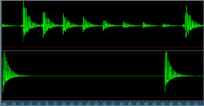
A plot of the output of the recirculating delay line echo patch is shown in the figure below. You can see that the echo time is about 0.5 seconds, and that the signal is degraded somewhat.
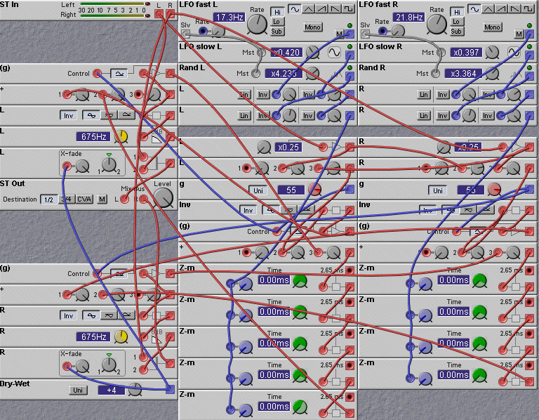
The following figure shows a reverb patch based on the recirculating delay line technique. It uses the well-known Gardner reverb algorithm developed by William Gardner in his 1992 MIT Master's thesis. Details of the Gardner algorithm are available in many places on the web. The sound of this patch is quite bad, partly due to the low frequency response, partly due to the distorting effects of overlapping recirculation slots, and partly to the difficulty of finding suitable delay time settings to match those suggested by Gardner.