Next: Using LTP: Some Practical
Up: Practical Applications of Lie
Previous: Trajectory planning and control
Contents
Lie algebraic methods originally conceived as tools for the
analysis of nonlinear systems have also found application in nonlinear
filtering problems; the reader is referred to [23] for a
complete expository review. In the nonlinear filtering problem the
objective is to estimate the state of a stochastic process  which cannot be measured directly, but may be inferred from
measurements of a related observation process
which cannot be measured directly, but may be inferred from
measurements of a related observation process  .
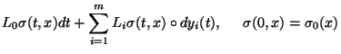
Typical filtering problems consider the following signal observation model:
.
Typical filtering problems consider the following signal observation model:
where  and
and  are
are  and
and  valued processes, respectively, and
  and
and  have components which are independent, standard Brownian processes. Furthermore,
  and
and  are assumed to be smooth functions.
Essential for the estimation of the state is the conditional probability density of the state,
are assumed to be smooth functions.
Essential for the estimation of the state is the conditional probability density of the state, 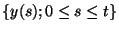 , given the observation
 . It is well known, see [10], that is obtained by normalizing a function
  which is the solution of the Duncan-Mortensen-Zakai (DMZ) bilinear, stochastic, partial differential equation:
where  denotes the Fisk-Stratonovitch differential of the observation process , the differential operator
 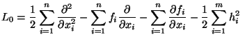 , given by:
 |
|
|
(22) |
is defined on the space of smooth functions
 on with compact support, and where
  is the operator of multiplication by
  ,
,  . Here,
 is the probability density of the initial point
  , and
, and
 denotes the space of nonnegative bounded measures on .
A particularly useful concept associated with the DMZ equation is the estimation Lie algebra, as introduced in [5], which is defined as the Lie algebra generated by the differential operators
denotes the space of nonnegative bounded measures on .
A particularly useful concept associated with the DMZ equation is the estimation Lie algebra, as introduced in [5], which is defined as the Lie algebra generated by the differential operators
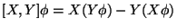 (the Lie product of operators is calculated in a standard way, i.e.
![$[X,Y]\phi=X(Y\phi)-Y(X\phi)$](img285.png) , for any smooth function
, for any smooth function  ). The structure and dimensionality of the estimation Lie algebra is directly related to the existence of a finite dimensional recursive filter for the computation of , see [23]. It has been shown that if the estimation Lie algebra can be identified with a Weyl algebra of any order, then no non-constant statistics exist for the computation of the conditional density with a finite dimensional filter; see references in [23]. In this context, the LTP package is helpful in the computation of the generators for the Weyl algebras as it permits to compute the Lie product in a coordinate independent fashion.
In the special case when the estimation Lie algebra is finite dimensional and solvable, (see [43] for the definition of solvability), the DMZ equation can be solved via an extension of the Wei-Norman formalism. Such a construction will be illustrated by an example employing the Lie tools package.
). The structure and dimensionality of the estimation Lie algebra is directly related to the existence of a finite dimensional recursive filter for the computation of , see [23]. It has been shown that if the estimation Lie algebra can be identified with a Weyl algebra of any order, then no non-constant statistics exist for the computation of the conditional density with a finite dimensional filter; see references in [23]. In this context, the LTP package is helpful in the computation of the generators for the Weyl algebras as it permits to compute the Lie product in a coordinate independent fashion.
In the special case when the estimation Lie algebra is finite dimensional and solvable, (see [43] for the definition of solvability), the DMZ equation can be solved via an extension of the Wei-Norman formalism. Such a construction will be illustrated by an example employing the Lie tools package.
Next: Using LTP: Some Practical
Up: Practical Applications of Lie
Previous: Trajectory planning and control
Contents
Miguel Attilio Torres-Torriti
2004-05-31