Scott McCloskey
ICSG 755 - Neural Networks and Machine Learning
Winter 1999-2000
Research Paper
Probabilistic Reasoning and Bayesian Networks
Much of the current research in the field of Computer Science is centered about the various methods of machine learning. In a broad sense, machine learning is an attempt to teach computers to use reasoning methods similar to those employed by humans. In the study of machine learning, it becomes obvious that most of these methods are founded in mathematical fields. Neural Networks, for instance, use a learning algorithm derived from statistics. Other types of machine learning such as face recognition are based upon the principals of linear algebra. It should come as no surprise, then, that another major branch of mathematics, probability theory, has yielded its own type of machine learning, Bayesian Networks. It is the purpose of this paper to describe the underlying concepts and theory that make Bayesian Networks valid, describe some of the strengths and weaknesses of Bayesian Networks relative to other popular methods of machine learning, and a specific example of a Bayesian Network in action.
Before moving on to the technical discussion, however, it is important to discuss the motivations for probabilistic reasoning, the method of reasoning that is used with Bayesian Networks. The three obvious reasons are as follows:
In addition to these three reasons, there is a fourth reason that may be equally valid: laziness. It is easy to imagine a problem whose number of influencing factors is large enough to make deterministic reasoning impractical.
The basic concept that underlies probabilistic reasoning is the idea that we can measure the belief that propositions are true, or that events will take place. We then use probability theory as a formal method of manipulating these degrees of belief.
The basic measure of our belief in a certain proposition will be the function P(A), which measures our belief in the proposition A. P(A) is a real-valued function on the interval [0, 1], with P(A) = 1 meaning that A is always true, and P(A) = 0 meaning that A is always false. Other values in the interval indicate the firmness of our belief that A is true.
Before moving on to the basic axioms of probability, it is important to mention the difference between a proposition and a variable. The character A, as used in the previous paragraph, represents a preposition, which could be something like 'the minimum temperature today was 5 degrees', or 'Bill Clinton is the president of the United States'. Prepositions can also be used to indicate the values of variables. For instance, if X is a variable whose possible values are x1, x2, … xn, then we see that X=x1, X=x2, …. X=xn are all propositions. Propositions can also be constructed from other propositions by the use of the logical operators OR (represented by v), AND (^), and NEGATION (~).
The basic axioms, then, are as follows:
We now introduce the concept of conditional probabilities and the related consequences. Conditional probabilities give a measure of how our beliefs in certain propositions are changed by the introduction of related knowledge. We represent conditional probabilities as P(A | B), which reads 'the probability of A, given that B is true.' For example, if we let T represent the proposition 'the temperature in Rochester will exceed 32 degrees today', and W represent 'today is a day in January', we can consider the probability P(T | W). The difference between P(T) and P(T | W) represents how we adjust our beliefs about temperature in light of the fact that it is winter.
To gain further intuition about conditional probabilities, consider these formulas:
This brings us to the notion of conditional dependence and independence, concepts that are fundamental in the construction and use of Bayesian Networks. We say that a proposition (A) is conditionally dependent upon another (B) if the knowledge that B is true changes our belief that A is true. The example of winter temperatures mentioned above is an example of a conditional dependence.
Conversely, we say that A is conditionally independent of B if the knowledge that B is true has no effect on our belief in A. In terms of our notation, P(A | B) = P(A). As an example, let T be the proposition 'the temperature in Rochester will exceed 35 degrees today', and let R be 'today is Thursday'. Our intuition would indicate that, since the day of the week has no impact on the temperature, T is conditionally independent of R, and consequentially P(T | R) = P(T).
Conditional probabilities give rise to a number of new results:
With all this formalism in place, our attention is turned to representing knowledge about a problem in an efficient and useful way. To do this, we use a Bayesian Network. The basic idea of such a network is to represent all of the random variables involved in the problem, along with the conditional dependencies between these variables.
Formally, a Bayesian Network is a directed acyclic graph with each vertex representing a random variable in the problem space. An edge is drawn from vertex A to B if B is conditionally dependant on A. Consequentially, the existence of a directed path from A to B indicates B's conditional dependence on A (note that this path may involve more than one edge). Conversely, B is conditionally independent of A if there is no directed path from A to B. Vertex A is said to be a parent of vertex B if there is a directed edge from A to B in the graph.
The other necessary component of a Bayesian Network is an encoding of the probabilistic information necessary to compute probabilities of interest. A conditional probability is stored for each variable given all possible values of its parents. Verticies without parents will have tables the only entry of which will be its observed probability. This is typically done by statistical observation, which requires a sort of training set from which to learn strengths of dependencies.
As an example, consider the problem of selling car insurance. A car insurance salesperson is interested in determining the probability that a specific person will be involved in a car accident. This salesperson determines that there are two factors that influence the probability of an individual getting in an accident: whether or not the person lives in a big city, and whether or not the person is accident-prone (which might, in turn, be based on other evidence. For simplicity's sake, assume that the salesman can measure whether or not someone is accident-prone). Furthermore, we assume that living in a big city and being accident-prone are mutually conditionally independent. Thus we have three boolean variables, H (the person will have an accident), B (the person lives in a big city), and A (the person is accident-prone). The Bayesian Network for this problem would look like:
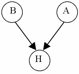
The edges in this graph to H from both B and A indicate H's conditional dependence on the two variables.
The next step in the construction of the network is finding the probabilities of each node given its parents. Let us assume that the salesperson has determined that
This completes the construction of the Bayesian Network for this problem.
Once constructed, Bayesian Networks can be used to reason in two different ways. The first method involves top-down reasoning, and is also known as predictive reasoning because it works from basic information (whether or not someone lives in a big city) and tries to predict behavior (whether or not the person will get in an accident). This method typically involves the use of the chain and addition rules to determine to resulting probability. An example of the predictive reasoning in our insurance example would be determining P(H | B), or the probability that a person who lives in a big city will get in an accident, without any knowledge of whether or not the individual is accident prone. We apply the addition rule to determine that
P(H | B) = P (H | B ^ A) * P(A) + P (H | B ^ ~A) * P(~A) = 0.6 * 0.3 + 0.3 * 0.7 = 0.39
The second type of reasoning involves bottom-up reasoning, and is also known as diagnostic reasoning because it works from symptoms (the person had an accident) to determine causes (whether or not the person is accident-prone). This method typically involves the use of Bayes Rule, the Product Rule, and conditional independence.
An example would be determining the probability that an individual lives in a big city given that s/he doesn't get in an accident, which is P(B|~H). By Bayes Rule, we find that
P(B | ~H) = P(B) * P(~H | B) / P(~H) = 0.5 * P(~H | B)/ P(~H)
By the addition rule, we can determine easily that P(~H) = 0.71.
Now we need to find P(~H | B), which comes out of the definition of conditional probability
P(~H | B) = P(~H ^ B) / P(B) = ( P(~H ^ B ^ A) + P(~H ^ B ^ ~A) ) / P(B)
Which reduces the problem to finding P(~H ^ B ^ A) and P(~H ^ B ^ ~A), which can be found as follows:
P(~H ^ B ^ A)
= P(~H | B ^ A) * P(B ^ A) by product rule
= P(~H | B ^ A) * P(B | A) * P(A) by product rule
= P(~H | B ^ A) * P(B) * P(A) by conditional independence of B given A
= 0.6 * 0.5 * 0.3 = 0.06
Similarly, P(~H ^ B ^ ~A) = 0.245, completing set of necessary probabilities.
P(~H | B) = ( P(~H ^ B ^ A) + P(~H ^ B ^ ~A) ) / P(B) = (0.245 + 0.06) / 0.5 = 0.61
P(B | ~H) = 0.5 * P(~H | B)/ P(~H) = 0.5 * 0.61 / 0.71 = 0.43
Thus completing the initial task of finding P(B | ~H).
From these two examples we see that one of the important strengths of Bayesian Networks is the fact that it provides a basis for reasoning in two very different ways.
Like other methods of machine learning, Bayesian Networks have been found to be useful for a significant number of applications. There are, however, characteristic strengths and weaknesses that Bayesian Network approaches have compared to other methods of machine learning.
Perhaps the most significant disadvantage of an approach involving Bayesian Networks is the fact that there is no universally accepted method for constructing a network from data. There are a number of efforts underway to come up with such methods, but the literature indicates that no clear winner has emerged to this point1. Two specific weaknesses come out of this lack, the first being that the design of a Bayesian Net requires a comparatively large amount of effort. A resulting problem is the fact that Bayesian Networks can only exploit causal influences that are recognized by the person programming it. Neural Networks, on the other hand, have the advantage of being able to learn any patterns, and aren't limited by the person programming them.
This disadvantage, though, is simultaneously an advantage over a neural network approach. In the training of neural networks there is no guarantee that all of the domain specific information is being used and, furthermore, inspecting for specific features is highly nontrivial. Bayesian networks, on the other hand, can be easily inspected to determine whether or not a certain feature of data is being taken into consideration, and can be forced to include that feature if necessary2. Because of this, Bayesian Networks can be guaranteed to exploit all known features of a problem.
A related advantage is that Bayesian Networks are more easily extensible than other machine learning methods. The addition of a new piece of evidence into a Bayesian Network would require only the addition of a fairly small number of probabilities, in addition to a fairly small number of edges in the graph. This is a steep contrast to expert systems, where the addition of a new piece of evidence requires a great deal of effort.
Perhaps the biggest advantage of an approach using Bayesian Networks is the fact that they can be used to reason in the two different directions, as mentioned previously. Because of this strength, Bayesian Networks are a more viable method for modeling certain cognitive functions3. Most neural networks, by contrast, only produce meaningful output in the feedforward direction, thus requiring two nets to do the job of a single Bayesian Network.
Another advantage of a Bayes Network is the fact that the output is explicitly a probability. In order to change the output of the network from a probability to a deterministic output, a threshold needs to be set. Neural networks, by contrast, output values that can be interpreted in a number of different ways. The disadvantage of the neural network approach is that these output values don't come with any confidence measure. A gross sense of confidence in a neural network approach can be found by (in the case of a "winner takes all approach") determining the difference between the two largest outputs, but there is little assurance that this translates into a reasonable confidence measure. Confidences in the outputs of a Bayes Network, on the other hand, are explicit in the output. If a Bayes Network's output threshold is set to 0.75, a network output of 0.79 can be classified as a positive result with low certainty.
Another strength of a Bayesian Network approach is the utility of the graph itself. Of high importance is the fact that the graph is a compact representation of the knowledge surrounding the system4. Due to their graphical nature, Bayes Networks are useful to both people and computers whereas a neural network is essentially unreadable to humans.
Recently, a number of researchers at Microsoft have attempted to try and use a Bayesian Network to identify junk e-mail such as advertisements. In order to do so, they needed to come up with features that could act as evidence in determining whether or not a specific piece of e-mail is junk. Their solution included three types of features: words, phrases, and domain-specific metadata. The phrases used were selected by the researchers based on experience, and included phrases such as "free money" and "big savings". The domain-specific metadata, also selected by the researchers, were things like the time of day that the message was sent (most junk mail is sent out en masse late at night when traffic is low). The third type of feature, specific words, were found by statistically analyzing pre-identified pieces of junk and relevant mail to determine words that are used more frequently in junk e-mail. The inclusion of these words helps, in part, to remove the disadvantage of only including features that were easily recognized by the designers.
An important consideration in this experiment turned out to be the setting of the final threshold that determined whether or not a piece of e-mail was garbage. The assumption was made that it is preferable to err in classifying junk mail as meaningful, rather than accidentally delete something important. In accordance with this, the threshold they set was a 99.9% confidence that a piece of mail was junk. With this threshold, the network managed to classify all good e-mail as such, while misclassifying only a small amount of junk mail as meaningful (3.8% of the mail classified as good was actually junk). This test was considered a success as it had met its primary goal: reducing the amount of junk e-mail received while ensuring that all good e-mail was successfully classified as such.
As the above indicate, Bayesian Networks are a useful method of machine learning when applied correctly. Ultimately, though, the requirements of, and the person undertaking, the specific problem determine the approach taken. This decision is ideally based on the advantages and disadvantages of a Bayesian Network solution as compared to the other viable methods of machine learning, as outlined in this paper. Future work is important to the field, meanwhile, as methods for learning nets from data are refined. Such methods will not only simplify the creation of useful Bayesian Networks, but also have the potential of identifying features in data that go undetected by human researchers.
References
Works Cited
M. Sahami, S. Dumais, D. Heckerman, and E. Horvitz. A Bayesian Approach to Filtering
Junk E-mail. AAAI'98 Workshop on Learning for Text Categorization, July 27, 1998, Madison, Wisconsin. Available online at http://www.research.microsoft.com/~heckerman/spam98.ps
Perl, Judea. Bayesian Networks. UCLA Technical Report (R-246), Revision I, July
1997.
Heckerman, David. A Tutorial on Learning with Bayesian Networks.
Presented at The Twelfth International Conference on Machine Learning, Tahoe City, CA, July 9, 1995. Revised November 1996